3.2.1. Reactor pin cell

import os
import h5py
import numpy as np

3.2.1.1. Using this Notebook

Before running this example, make sure that the Python module of OpenSn was installed.

3.2.1.1.1. Converting and Running this Notebook from the Terminal

To run this notebook from the terminal, simply type:

jupyter nbconvert --to python --execute <notebook_name>.ipynb.

To run this notebook in parallel (for example, using 4 processes), simply type:

mpiexec -n 4 jupyter nbconvert --to python --execute <notebook_name>.ipynb.

from mpi4py import MPI
size = MPI.COMM_WORLD.size
rank = MPI.COMM_WORLD.rank

if rank == 0:
    print(f"Running with {size} MPI processors.")

3.2.1.2. Import Requirements

Import required classes and functions from the Python interface of OpenSn. Run this notebook from an environment where the pyopensn package is importable.

from pyopensn.mesh import FromFileMeshGenerator
from pyopensn.xs import MultiGroupXS
from pyopensn.aquad import GLCProductQuadrature2DXY
from pyopensn.solver import DiscreteOrdinatesProblem, PowerIterationKEigenSolver
from pyopensn.fieldfunc import FieldFunctionGridBased, FieldFunctionInterpolationVolume
from pyopensn.logvol import RPPLogicalVolume

from pyopensn.context import UseColor, Finalize

3.2.1.2.1. Disable colorized output

UseColor(False)

3.2.1.3. Mesh

We load a reactor pin lattice (.obj file). The mesh and its block IDs are shown below:

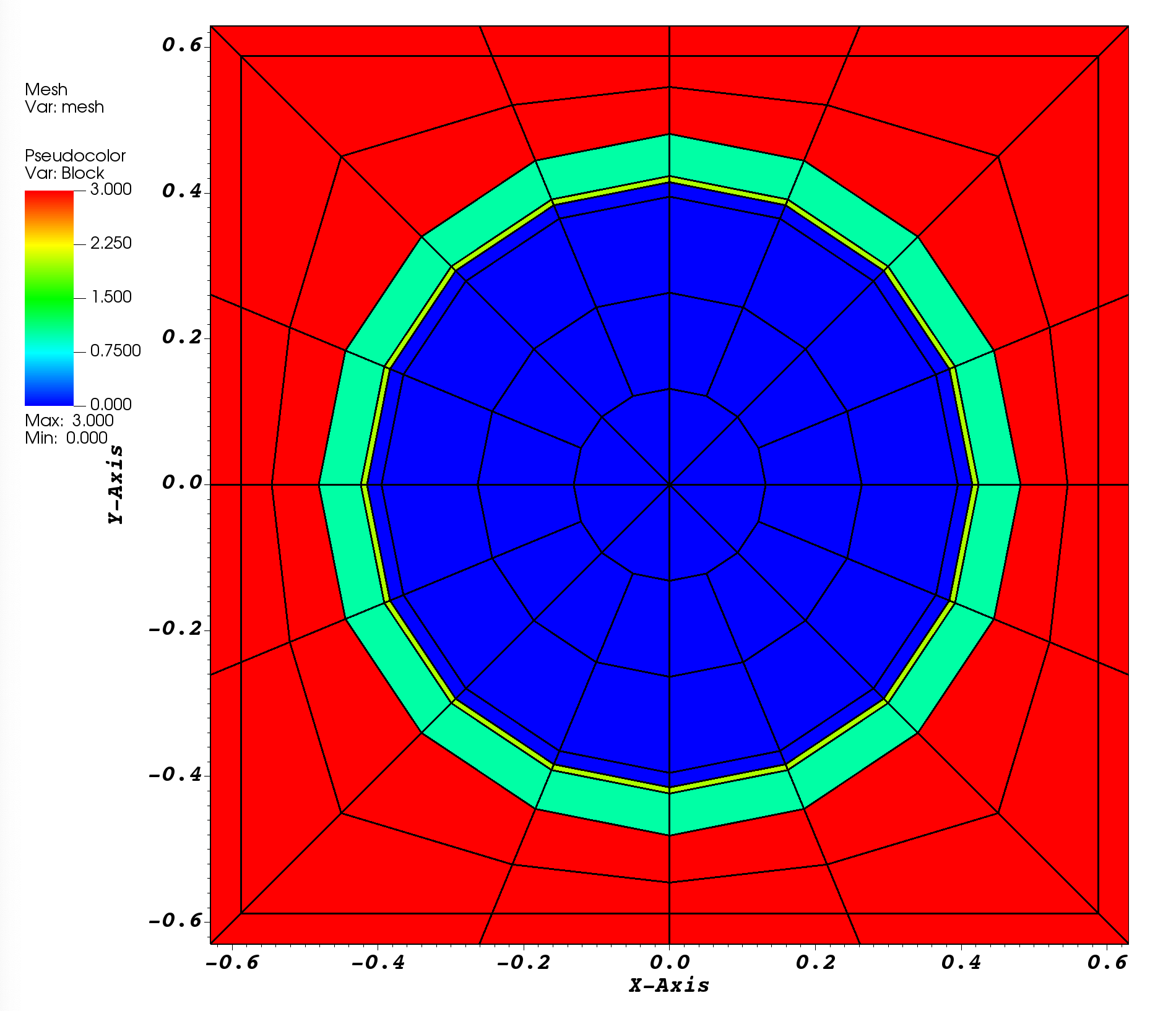
div>

meshgen = FromFileMeshGenerator(filename="pincell.obj")
grid = meshgen.Execute()
grid.SetOrthogonalBoundaries()
grid.ExportToPVTU("pincell_mesh")

3.2.1.4. Cross Sections

We load 361-group cross sections that were generated using OpenMC.

xs_filepath = "./mgxs_2B_one_eighth_SHEM-361.h5"

with h5py.File(xs_filepath, "r") as h5_file:
    group_edges = np.asarray(h5_file.attrs["group structure"])
    num_groups = int(h5_file.attrs["energy_groups"])

if group_edges.size != num_groups + 1:
    raise ValueError("The number of group edges is inconsistent with the number of energy groups.")

h5_mat_names = [
    "fuel",
    "fuel clad",
    "fuel gap",
    "moderator",
]

xs_dict = {}
xs_list = []
for name in h5_mat_names:
    xs_dict[name] = MultiGroupXS()
    xs_dict[name].LoadFromOpenMC(xs_filepath, name, 294.0)
    xs_list = np.append(xs_list, xs_dict[name])

block_ids = [i for i in range(0, len(xs_list))]

scat_order = 3  # xs_list[0].scattering_order

if any(xs.num_groups != num_groups for xs in xs_list):
    raise ValueError("The HDF5 energy-group metadata is inconsistent with the cross sections.")

3.2.1.5. Angular Quadrature

We create a product Gauss-Legendre-Chebyshev angular quadrature and pass the total number of polar cosines (here n_polar = 2) and the number of azimuthal subdivisions in four quadrants (n_azimuthal = 4).

For more accurate results, we suggest using n_polar = 8 and n_azimuthal = 32

pquad = GLCProductQuadrature2DXY(n_polar=2, n_azimuthal=4, scattering_order=scat_order)

3.2.1.6. Linear Boltzmann Solver

3.2.1.6.1. Options for the Linear Boltzmann Problem (LBS)

group_sets = [
    {
        "groups_from_to": (0, num_groups - 1),
        "angular_quadrature": pquad,
        "angle_aggregation_type": "polar",
        "inner_linear_method": "classic_richardson",
        "l_abs_tol": 1.0e-5,
        "l_max_its": 300,
    }
]

bound_conditions = [
    {"name": "xmin", "type": "reflecting"},
    {"name": "xmax", "type": "reflecting"},
    {"name": "ymin", "type": "reflecting"},
    {"name": "ymax", "type": "reflecting"},
]

xs_mapping = [
    {"block_ids": [0], "xs": xs_list[0]},
    {"block_ids": [1], "xs": xs_list[1]},
    {"block_ids": [2], "xs": xs_list[2]},
    {"block_ids": [3], "xs": xs_list[3]}
]

phys = DiscreteOrdinatesProblem(
    mesh=grid,
    num_groups=num_groups,
    groupsets=group_sets,
    xs_map=xs_mapping,
    boundary_conditions=bound_conditions,
    options={
        "verbose_inner_iterations": True,
        "verbose_outer_iterations": True,
        "use_precursors": False,
        "power_default_kappa": 1.0,
        "save_angular_flux": False,
    },
)

3.2.1.6.2. Putting the Linear Boltzmann Solver Together

We then create the physics solver, initialize it, and execute it.

k_solver = PowerIterationKEigenSolver(problem=phys, k_tol=1.0e-14)
k_solver.Initialize()
k_solver.Execute()

keff = k_solver.GetEigenvalue()

if rank ==0:
    print(f"Eigenvalue = {keff}")

3.2.1.7. Post-Processing via Field Functions

fflist = phys.GetScalarFluxFieldFunction()
vtk_basename = "pin_cell"
FieldFunctionGridBased.ExportMultipleToPVTU([fflist[g] for g in range(num_groups)], vtk_basename)

3.2.1.8. Post-processing: Extract the average flux in a portion of the domain

We create an edit zone (logical volume) that is the entire domain.

We request the average (keyword "avg") of the scalar flux over the edit zone, for each group.

logvol_whole_domain = RPPLogicalVolume(infx=True, infy=True, infz=True)

flux = np.zeros(num_groups)
for g in range(0, num_groups):
    ffi = FieldFunctionInterpolationVolume()
    ffi.SetOperationType("sum")
    ffi.SetLogicalVolume(logvol_whole_domain)
    ffi.AddFieldFunction(fflist[g])
    ffi.Execute()
    flux[g] = ffi.GetValue()

flux /= np.sum(flux)

# OpenMC stores group boundaries in ascending energy order.
E = np.flip(group_edges)
# Compute the group widths.
dE = -np.diff(E)
# Compute the group midpoints.
Emid = E[:-1] + dE/2

import matplotlib.pyplot as plt

if rank == 0:
    fig, ax = plt.subplots()
    y = Emid * flux / dE
    y = np.insert(y, 0, y[0])

    ax.semilogx(E, y, drawstyle="steps", label="Flux")
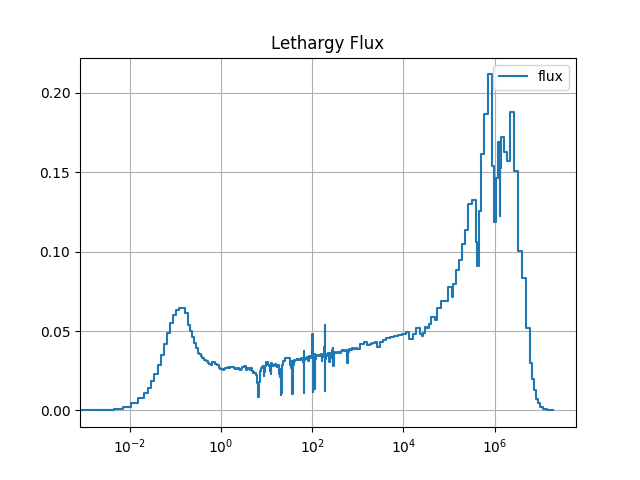
    ax.set_title("Lethargy Flux")
    ax.set_xlabel("Energy (eV)", loc="center")
    ax.set_ylabel("Normalized flux per unit lethargy")
    ax.legend()
    ax.grid()
    fig.tight_layout()
    # fig.savefig("./images/pincell_lethargy_spectrum.png")
    # plt.show()

    fig, ax = plt.subplots()
    y = flux / dE
    y = np.insert(y, 0, y[0])

    ax.loglog(E, y, drawstyle="steps", label="Flux")
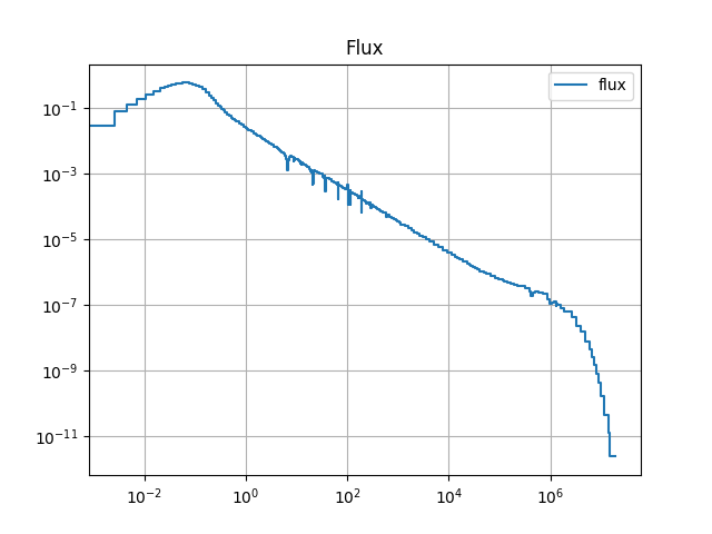
    ax.set_title("Flux")
    ax.set_xlabel("Energy (eV)", loc="center")
    ax.set_ylabel(r"Normalized flux per unit energy (eV$^{-1}$)")
    ax.legend()
    ax.grid()
    fig.tight_layout()
    # fig.savefig("./images/pincell_spectrum.png")
    # plt.show()

The resulting spectra are shown below:

3.2.1.9. Finalize (for Jupyter Notebook only)

In Python script mode, PyOpenSn automatically handles environment termination. However, this automatic finalization does not occur when running in a Jupyter notebook, so explicit finalization of the environment at the end of the notebook is required. Do not call the finalization in Python script mode, or in console mode.

Note that PyOpenSn’s finalization must be called before MPI’s finalization.

MPI.COMM_WORLD.Barrier()

from IPython import get_ipython

def finalize_env():
    Finalize()
    MPI.Finalize()

ipython_instance = get_ipython()
if ipython_instance is not None:
    ipython_instance.events.register("post_execute", finalize_env)