3.4.2. Switching From Steady-State to Transient to Steady-State in OpenSn
3.4.2.1. Using this Notebook
Before running this example, make sure the Python module of OpenSn is available in your environment.
3.4.2.1.1. Converting and Running this Notebook from the Terminal
To run this notebook from the terminal, use:
jupyter nbconvert --to python --execute source_step_steady_to_transient_to_steady.ipynb
To run in parallel (for example, 4 ranks):
mpiexec -n 4 jupyter nbconvert --to python --execute source_step_steady_to_transient_to_steady.ipynb
3.4.2.2. Import Requirements
Import required classes and functions from the Python interface of OpenSn. Run this notebook from an environment where the pyopensn package is importable.
3.4.2.2.1. Disable colorized output
For notebook rendering, plain (non-colorized) output is typically easier to read.
[ ]:
import math
import os
import sys
import ctypes
from pathlib import Path
import matplotlib.pyplot as plt
if "opensn_console" not in globals():
    from mpi4py import MPI
    size = MPI.COMM_WORLD.size
    rank = MPI.COMM_WORLD.rank
    # In notebooks, __file__ is typically undefined. Prefer cwd as the tutorial dir.
    tutorial_dir = Path(__file__).resolve().parent if "__file__" in globals() else Path.cwd()
    # If launched from repo root (or another directory), recover the tutorial directory.
    if not (tutorial_dir / "xs1g_prompt_crit.cxs").exists():
        candidate = Path.cwd() / "doc/source/tutorials/problems/transient"
        if candidate.exists():
            tutorial_dir = candidate
    repo_root = None
    build_dir = None
    # Prefer normal environment import (e.g., site-packages), then fall back to local build.
    try:
        import pyopensn
    except ImportError:
        # Find repo root robustly by walking upward.
        for p in [tutorial_dir, *tutorial_dir.parents]:
            has_src_pyopensn = (p / "pyopensn").exists() and (p / "CMakeLists.txt").exists()
            has_bld_pyopensn = (p / "build" / "pyopensn").exists()
            if has_bld_pyopensn or has_src_pyopensn:
                repo_root = p
                break
        if repo_root is None:
            repo_root = tutorial_dir
        build_dir = repo_root / "build"
        if (build_dir / "pyopensn").exists():
            # Avoid stale module path order issues.
            sys.path = [p for p in sys.path if p not in (str(build_dir), str(repo_root))]
            sys.path.insert(0, str(build_dir))
        # Preload local libopensn if available (Linux/macOS).
        lib_candidates = (
            build_dir / "libopensn.so",
            build_dir / "libopensn.dylib",
            build_dir / "lib" / "libopensn.so",
            build_dir / "lib" / "libopensn.dylib",
        )
        for lib_path in lib_candidates:
            if lib_path.exists():
                ctypes.CDLL(str(lib_path), mode=ctypes.RTLD_GLOBAL)
                break
        import pyopensn
        # If we used fallback import, ensure we loaded from local build.
        pyopensn_path = Path(pyopensn.__file__).resolve()
        expected_parent = (build_dir / "pyopensn").resolve()
        if expected_parent.exists() and expected_parent not in pyopensn_path.parents:
            raise RuntimeError(
                f"Imported pyopensn from unexpected location: {pyopensn_path}. "
                f"Expected under {expected_parent}"
            )
    from pyopensn.context import Finalize
    from pyopensn.mesh import OrthogonalMeshGenerator
    from pyopensn.xs import MultiGroupXS
    from pyopensn.source import VolumetricSource
    from pyopensn.aquad import GLProductQuadrature1DSlab
    from pyopensn.solver import (
        DiscreteOrdinatesProblem,
        SteadyStateSourceSolver,
        TransientSolver,
    )
    from pyopensn.post import VolumePostprocessor
else:
    # In opensn_console mode, solver symbols are preloaded by the runtime.
    rank = 0
def total_flux(problem):
    """Volume-integrated scalar flux summed over all groups."""
    integral = VolumePostprocessor(problem=problem, value_type="integral")
    integral.Execute()
    return float(integral.GetValue()[0].sum())
3.4.2.3. Mesh
We construct a 1D Cartesian mesh (10 cells on ([0,1])) so this tutorial focuses on workflow behavior rather than geometry complexity.
[ ]:
num_cells_1d = 10
L = 1.0
dx = L / num_cells_1d
nodes = [i * dx for i in range(num_cells_1d + 1)]

meshgen = OrthogonalMeshGenerator(node_sets=[nodes])
grid = meshgen.Execute()
3.4.2.4. Material IDs
Assign a single material ID (0) to all cells.
[ ]:
grid.SetUniformBlockID(0)
3.4.2.5. Cross Sections
Use a one-group pure absorber model:
For this setup, the steady source-driven solution is
.
The checks below use the volume-integrated scalar flux, summed over groups,
so the steady-state reference is \(\Phi_{ss} = V\,Q/\Sigma_t\), where \(V = L\) is the slab volume per unit transverse area.
[ ]:
sigma_t = 1.0
sigma_s = 0.0
q0 = 2.0  # initial steady-state source strength
q1 = 3.0  # post-step source strength
domain_volume = L  # slab volume per unit transverse area

dt = 0.1
t_end = 0.5

xs = MultiGroupXS()
xs.CreateSimpleOneGroup(sigma_t, sigma_s, 1.0)

src0 = VolumetricSource(block_ids=[0], group_strength=[q0], start_time=0.0, end_time=1.0e9)
src1 = VolumetricSource(block_ids=[0], group_strength=[q1], start_time=0.0, end_time=1.0e9)
3.4.2.6. Angular Quadrature
Use a low-order 1D slab quadrature.
[ ]:
pquad = GLProductQuadrature1DSlab(n_polar=4, scattering_order=0)
3.4.2.7. Linear Boltzmann Solver
Create one DiscreteOrdinatesProblem object that is reused across all three phases:
steady-state source solve with
Q0,transient with source stepped to
Q1,final steady-state source solve at
Q1.
[ ]:
phys = DiscreteOrdinatesProblem(
    mesh=grid,
    num_groups=1,
    groupsets=[
        {
            "groups_from_to": (0, 0),
            "angular_quadrature": pquad,
            "inner_linear_method": "petsc_richardson",
            "l_abs_tol": 1.0e-8,
            "l_max_its": 200,
        }
    ],
    xs_map=[{"block_ids": [0], "xs": xs}],
    volumetric_sources=[src0],
    boundary_conditions=[
        {"name": "zmin", "type": "reflecting"},
        {"name": "zmax", "type": "reflecting"},
    ],
    options={
        "save_angular_flux": True,
        "verbose_inner_iterations": False,
        "verbose_outer_iterations": False,
    },
)
3.4.2.8. Steady-State Solve (Initial Source (Q_0))
Solve a source-driven steady-state problem and compare the volume-integrated flux against
.
[ ]:
steady0 = SteadyStateSourceSolver(problem=phys)
steady0.Initialize()
steady0.Execute()

flux_ss0_num = total_flux(phys)
flux_ss0_ana = domain_volume * q0 / sigma_t

if rank == 0:
    print(f"Initial steady numeric total flux = {flux_ss0_num:.8e}")
    print(f"Initial steady analytic total flux = {flux_ss0_ana:.8e}")
3.4.2.9. Transition to Transient Mode and Step Source to (Q_1)
Switch to time-dependent mode, initialize from the existing steady state, and replace the volumetric source with the stepped value Q1.
[ ]:
phys.SetTimeDependentMode()
transient_solver = TransientSolver(problem=phys, dt=dt, theta=1.0, initial_state="existing")
transient_solver.Initialize()

phys.SetVolumetricSources(clear_volumetric_sources=True)
phys.SetVolumetricSources(volumetric_sources=[src1])
3.4.2.10. Advance in Time (Transient Solve)
Advance from (t=0) to (t=t_{end}) using backward Euler.
[ ]:
time_history = [phys.GetTime()]
flux_history = [flux_ss0_num]

step = 0
while phys.GetTime() < t_end:
    t_before = phys.GetTime()
    transient_solver.Advance()
    t_after = phys.GetTime()
    flux_now = total_flux(phys)
    time_history.append(t_after)
    flux_history.append(flux_now)
    if rank == 0:
        print(
            f"step={step:03d}, t={t_before:.4f}->{t_after:.4f}, total flux={flux_now:.8e}"
        )
    step += 1

flux_td_num = total_flux(phys)
n_steps = step
3.4.2.11. Return to Steady-State Mode (Final Source (Q_1))
Switch back to steady-state mode and solve again with the same final source Q1. The final steady solution should satisfy
.
[ ]:
phys.SetSteadyStateMode()
steady1 = SteadyStateSourceSolver(problem=phys)
steady1.Initialize()
steady1.Execute()

flux_ss1_num = total_flux(phys)
flux_ss1_ana = domain_volume * q1 / sigma_t
3.4.2.12. Post-processing: Analytic Checks for the Full Workflow
For backward Euler with constant source (Q_1), the transient update is
.
With initial value
, after (N) steps:
The flux stays spatially uniform, so the volume-integrated flux is (\Phi`^N = V:nbsphinx-math:phi`^N). We compare:
transient numerical (\Phi`^N) vs analytic (V:nbsphinx-math:phi`^N),
final steady numerical (\Phi_{ss,1}) vs analytic (V Q_1/\Sigma_t).
[ ]:
r = 1.0 / (1.0 + sigma_t * dt)
flux_td_ana = flux_ss1_ana + (flux_ss0_ana - flux_ss1_ana) * (r ** n_steps)

err_td = abs(flux_td_num - flux_td_ana) / max(abs(flux_td_ana), 1.0e-16)
err_ss = abs(flux_ss1_num - flux_ss1_ana) / max(abs(flux_ss1_ana), 1.0e-16)

tol_td = 5.0e-3
tol_ss = 1.0e-3
ok = (err_td < tol_td) and (err_ss < tol_ss)

if rank == 0:
    print(f"Transient-end numeric total flux = {flux_td_num:.8e}")
    print(f"Transient-end analytic total flux = {flux_td_ana:.8e}")
    print(f"Final steady numeric total flux = {flux_ss1_num:.8e}")
    print(f"Final steady analytic total flux = {flux_ss1_ana:.8e}")
    print(f"Relative error (transient) = {err_td:.3e}")
    print(f"Relative error (steady)    = {err_ss:.3e}")
    print(f"SOURCE_STEP_WORKFLOW_OK {1 if ok else 0}")

assert ok, (
    f"Workflow check failed: err_td={err_td:.3e}, err_ss={err_ss:.3e}, "
    f"tol_td={tol_td:.3e}, tol_ss={tol_ss:.3e}"
)
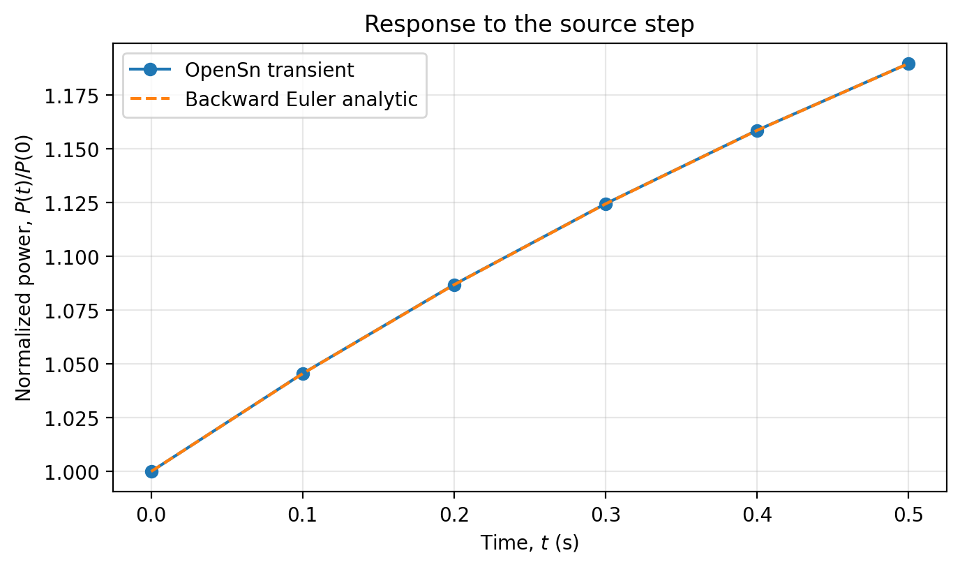
3.4.2.13. Flux amplitude history
This source-driven benchmark uses non-fissionable material, so it has no fission power. We measure the temporal response with the flux amplitude
computed with a VolumePostprocessor. A ratio of pointwise maxima, \(\max\phi(t)/\max\phi(0)\), follows a single group at a single location, so it is not defined for multigroup problems and changes meaning if the location of the maximum moves during the transient. The volume integral includes every group and every cell.
For a fissile transient, measure power with the volume-integrated fission rate instead, VolumePostprocessor(problem=phys, xs_multiplier="sigma_f"), as in the k-eigenvalue transient tutorial. The committed figure below was generated by this cell; uncomment fig.savefig(...) to regenerate it after changing the problem.
[ ]:
relative_amplitude = [flux / flux_ss0_num for flux in flux_history]
relative_amplitude_be = [
    (flux_ss1_ana + (flux_ss0_ana - flux_ss1_ana) * r**n) / flux_ss0_ana
    for n in range(len(time_history))
]

if rank == 0:
    fig, ax = plt.subplots(figsize=(7.0, 4.2))
    ax.plot(time_history, relative_amplitude, "o-", label="OpenSn transient")
    ax.plot(time_history, relative_amplitude_be, "--", label="Backward Euler analytic")
    ax.set_xlabel(r"Time, $t$ (s)")
    ax.set_ylabel(r"Normalized flux amplitude, $\Phi(t)/\Phi(0)$")
    ax.set_title("Response to the source step")
    ax.grid(alpha=0.3)
    ax.legend()
    fig.tight_layout()
    # fig.savefig("images/source_step_power_history.png", dpi=200, bbox_inches="tight")
    plt.close(fig)
    print(f"SOURCE_STEP_FINAL_NORMALIZED_AMPLITUDE {relative_amplitude[-1]:.8e}")
3.4.2.14. Finalize (for Jupyter Notebook only)
In Python script mode, PyOpenSn usually handles environment termination automatically. In Jupyter notebook mode, finalize explicitly only if your runtime requires it.
[ ]:
if "opensn_console" not in globals():
    from IPython import get_ipython

    if get_ipython() is not None:
        Finalize()
        MPI.Finalize()