3.5. Lebedev Quadrature

This set uses Lebedev quadrature points on the unit sphere.

To run the code, simply type: jupyter nbconvert --to python --execute <basename>.ipynb.

To convert it to a python file (named <basename>.py), simply type: jupyter nbconvert --to python <basename>.ipynb

import os
import sys
import numpy as np
from mpi4py import MPI

sys.path.append("../..")

from pyopensn.aquad import LebedevQuadrature3DXYZ
from pyopensn.context import UseColor, Finalize

UseColor(False)

3.5.1. Quadrature parameters

Here, we use a Lebedev Quadrature for three-dimensional geometries.

Lebedev quadrature sets differ from other sets in a few key ways.

1. There is a smaller amount of customization available when perscribing the set. The quadrature points are specified in literature, and OpenSn uses the standard scheme when refering to the quadrature orders.

2. These sets can include points that have an angular component equal to 0. The most straightforward example of this is the first order, which includes 6 points, all lying on the axial extremes +1 and -1 with the other two components equal to 0.

3. As a consequence of 2, the number of points in the 2D set is not equal to 1/2 the points of the 3D set.

OpenSn currently supports all orders up to 131; however, certain scattering-operator schemes do not support all sets. Currently, the Galerkin Methods are only supported up through order 101, and exclude orders 13, 25, and 27. The excluded orders are due to negative quadrature weights present in these sets, and thus an orthogonal basis with respect to quadrature integration does not make sense.

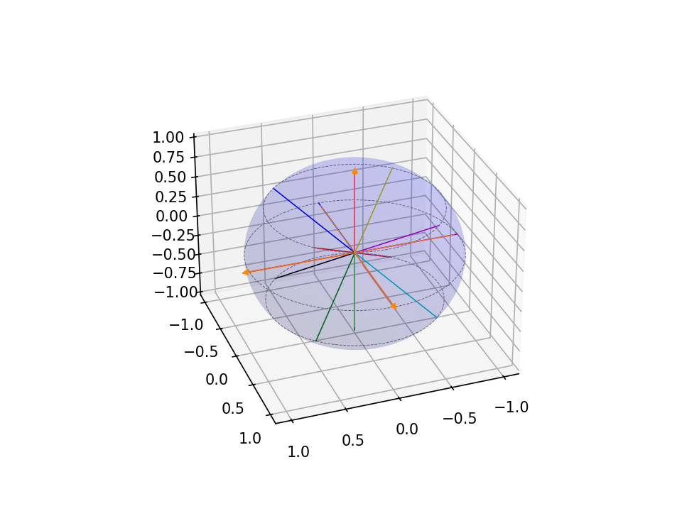
We pick a quadrature set of order 5, which yields 14 directions on the full sphere.

# Create a 3D Lebedev angular quadrature of order 5.
pquad = LebedevQuadrature3DXYZ(quadrature_order=5, scattering_order=0)

3.5.2. Retrieve directions

vec3_omegas = pquad.omegas

n_directions = len(vec3_omegas)
print('number of directions =',n_directions)
omegas = np.zeros((n_directions,3))

for d in range(n_directions):
    omegas[d,:] = [vec3_omegas[d].x, vec3_omegas[d].y, vec3_omegas[d].z]

dim = 3

3.5.3. Create a function to plot the quadrature

import matplotlib.pyplot as plt
from matplotlib.patches import FancyArrowPatch
from mpl_toolkits.mplot3d import proj3d
import itertools

colors = itertools.cycle(["r", "g", "b", "k", "m", "c", "y", "crimson"])

# Create figure with options
fig = plt.figure(dpi=150)
ax = fig.add_subplot(111, projection='3d')

# Transparent sphere data
u = np.linspace(0, 2 * np.pi, 100)
v = np.linspace(0, np.pi, 100)
x = np.outer(np.cos(u), np.sin(v))
y = np.outer(np.sin(u), np.sin(v))
z = np.outer(np.ones(np.size(u)), np.cos(v))
# Plot the surface
ax.plot_surface(x, y, z, color='b', alpha=0.1)

# Create a custom 3D arrow class
class Arrow3D(FancyArrowPatch):
    def __init__(self, xs, ys, zs, *args, **kwargs):
        # Initialize with dummy 2D points
        super().__init__((0, 0), (0, 0), *args, **kwargs)
        self._verts3d = xs, ys, zs

    def do_3d_projection(self, renderer=None):
        # Project 3D coordinates to 2D using the axes projection matrix
        xs3d, ys3d, zs3d = self._verts3d
        xs, ys, zs = proj3d.proj_transform(xs3d, ys3d, zs3d, self.axes.get_proj())
        self.set_positions((xs[0], ys[0]), (xs[1], ys[1]))
        # Return a numerical depth value (for example, the mean of the projected z-values)
        return np.mean(zs)

    def draw(self, renderer):
        # Perform projection using the axes' projection matrix
        xs3d, ys3d, zs3d = self._verts3d
        xs, ys, zs = proj3d.proj_transform(xs3d, ys3d, zs3d, self.axes.get_proj())
        self.set_positions((xs[0], ys[0]), (xs[1], ys[1]))
        return super().draw(renderer)


start = -1.0

# Create axes arrows
a = Arrow3D(
    [start, 1.1],
    [0, 0],
    [0, 0],
    mutation_scale=10,
    lw=0.5,
    arrowstyle="-|>",
    color="darkorange",
)
ax.add_artist(a)

a = Arrow3D(
    [0, 0],
    [start, 1.1],
    [0, 0],
    mutation_scale=10,
    lw=0.5,
    arrowstyle="-|>",
    color="darkorange",
)
ax.add_artist(a)

a = Arrow3D(
    [0, 0],
    [0, 0],
    [start, 1.1],
    mutation_scale=10,
    lw=0.5,
    arrowstyle="-|>",
    color="darkorange",
)
ax.add_artist(a)

# Plot quadrature directions by octant
n_octants = int(2 ** dim)
octant_colors = [next(colors) for _ in range(n_octants)]
for d in range(n_directions):
    om = omegas[d, :]
    # Determine octant index from signs of coordinates
    oc = (0 if om[0] >= 0 else 4) + (0 if om[1] >= 0 else 2) + (0 if om[2] >= 0 else 1)
    ax.plot3D([0, om[0]], [0, om[1]], [0, om[2]], c=octant_colors[oc], linewidth=0.75)

mu = omegas[:, -1]
polar_level = np.unique(mu)
for r in polar_level:
    x = np.sqrt(1 - r ** 2) * np.cos(u)
    y = np.sqrt(1 - r ** 2) * np.sin(u)
    z = r * np.ones_like(u)
    ax.plot3D(x, y, z, 'grey', linestyle="dashed", linewidth=0.5)

ax.view_init(30, 70)

# uncomment this line for interactive plot
# plt.show()

3.5.3.1. You should be getting this plot (saved here in the Markdown for convenience).

3.5.4. Finalize (for Jupyter Notebook only)

In Python script mode, PyOpenSn automatically handles environment termination. However, this automatic finalization does not occur when running in a Jupyter notebook, so explicit finalization of the environment at the end of the notebook is required. Do not call the finalization in Python script mode, or in console mode.

Note that PyOpenSn’s finalization must be called before MPI’s finalization.

from IPython import get_ipython

def finalize_env():
    Finalize()
    MPI.Finalize()

ipython_instance = get_ipython()
if ipython_instance is not None:
    ipython_instance.events.register("post_execute", finalize_env)