3.3. Triangular Quadrature

This set uses a Gauss-Legendre quadrature along the polar angle, with decreasing orders of Gauss-Chebyshev quadrature along the azimuthal angle as the polar angle moves away from the equatorial plane.

To run the code, simply type: jupyter nbconvert --to python --execute <basename>.ipynb.

To convert it to a python file (named <basename>.py), simply type: jupyter nbconvert --to python <basename>.ipynb

import os
import sys
import numpy as np
from mpi4py import MPI

sys.path.append("../..")

from pyopensn.aquad import GLCTriangularQuadrature2DXY
from pyopensn.context import UseColor, Finalize

UseColor(False)

3.3.1. Quadrature parameters

Here, we use a Triangular Quadrature for two-dimensional geometries.

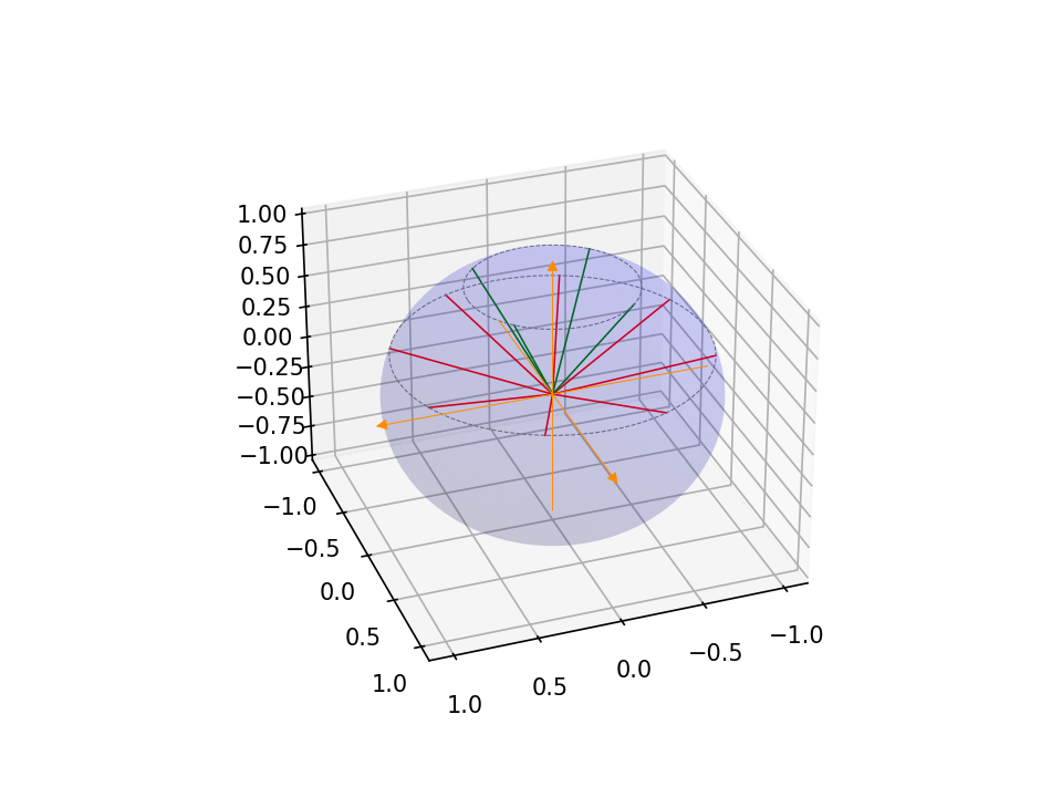
We pick a quadrature set with 4 polar angles. Unlike a product quadrature, the number of azimuthal angles varies per polar level: the maximum is \(2 \times N_{polar} = 8\) at the equator, decreasing by 4 (one per quadrant) for each polar level toward the pole. For 2D (upper hemisphere only with 2 polar levels), the azimuthal counts are [4, 8], giving a total of \(4 + 8 = 12\) directions.

# Create a 2D angular quadrature with 4 polar angles (triangular pattern).
tquad = GLCTriangularQuadrature2DXY(n_polar=4, scattering_order=0)

3.3.2. Retrieve directions

vec3_omegas = tquad.omegas

n_directions = len(vec3_omegas)
print('number of directions =',n_directions)
omegas = np.zeros((n_directions,3))

for d in range(n_directions):
    omegas[d,:] = [vec3_omegas[d].x, vec3_omegas[d].y, vec3_omegas[d].z]

dim = 2

3.3.3. Create a function to plot the quadrature

import matplotlib.pyplot as plt
from matplotlib.patches import FancyArrowPatch
from mpl_toolkits.mplot3d import proj3d
import itertools

colors = itertools.cycle(["r", "g", "b", "k", "m", "c", "y", "crimson"])

# Create figure with options
fig = plt.figure(dpi=150)
ax = fig.add_subplot(111, projection='3d')

# Transparent sphere data
u = np.linspace(0, 2 * np.pi, 100)
v = np.linspace(0, np.pi, 100)
x = np.outer(np.cos(u), np.sin(v))
y = np.outer(np.sin(u), np.sin(v))
z = np.outer(np.ones(np.size(u)), np.cos(v))
# Plot the surface
ax.plot_surface(x, y, z, color='b', alpha=0.1)

# Create a custom 3D arrow class
class Arrow3D(FancyArrowPatch):
    def __init__(self, xs, ys, zs, *args, **kwargs):
        # Initialize with dummy 2D points
        super().__init__((0, 0), (0, 0), *args, **kwargs)
        self._verts3d = xs, ys, zs

    def do_3d_projection(self, renderer=None):
        # Project 3D coordinates to 2D using the axes projection matrix
        xs3d, ys3d, zs3d = self._verts3d
        xs, ys, zs = proj3d.proj_transform(xs3d, ys3d, zs3d, self.axes.get_proj())
        self.set_positions((xs[0], ys[0]), (xs[1], ys[1]))
        # Return a numerical depth value (for example, the mean of the projected z-values)
        return np.mean(zs)

    def draw(self, renderer):
        # Perform projection using the axes' projection matrix
        xs3d, ys3d, zs3d = self._verts3d
        xs, ys, zs = proj3d.proj_transform(xs3d, ys3d, zs3d, self.axes.get_proj())
        self.set_positions((xs[0], ys[0]), (xs[1], ys[1]))
        return super().draw(renderer)


start = -1.0

# Create axes arrows
a = Arrow3D(
    [start, 1.1],
    [0, 0],
    [0, 0],
    mutation_scale=10,
    lw=0.5,
    arrowstyle="-|>",
    color="darkorange",
)
ax.add_artist(a)

a = Arrow3D(
    [0, 0],
    [start, 1.1],
    [0, 0],
    mutation_scale=10,
    lw=0.5,
    arrowstyle="-|>",
    color="darkorange",
)
ax.add_artist(a)

a = Arrow3D(
    [0, 0],
    [0, 0],
    [start, 1.1],
    mutation_scale=10,
    lw=0.5,
    arrowstyle="-|>",
    color="darkorange",
)
ax.add_artist(a)

# The following code plots quadrature directions, colored by polar level
# to highlight the triangular pattern (fewer directions near the pole).
mu = omegas[:, -1]
polar_levels = np.unique(np.round(mu, decimals=10))
print("number of polar levels =", len(polar_levels))
for plevel in polar_levels:
    clr = next(colors)
    mask = np.abs(mu - plevel) < 1e-9
    dirs = omegas[mask]
    print(f"  mu = {plevel:.4f}: {len(dirs)} directions")
    for om in dirs:
        ax.plot3D([0, om[0]], [0, om[1]], [0, om[2]], c=clr, linewidth=0.75)

for r in polar_levels:
    x = np.sqrt(1 - r ** 2) * np.cos(u)
    y = np.sqrt(1 - r ** 2) * np.sin(u)
    z = r * np.ones_like(u)
    ax.plot3D(x, y, z, 'grey', linestyle="dashed", linewidth=0.5)

ax.view_init(30, 70)

# uncomment this line for interactive plot
# plt.show()

3.3.3.1. You should be getting this plot (saved here in the Markdown for convenience).

3.3.4. Finalize (for Jupyter Notebook only)

In Python script mode, PyOpenSn automatically handles environment termination. However, this automatic finalization does not occur when running in a Jupyter notebook, so explicit finalization of the environment at the end of the notebook is required. Do not call the finalization in Python script mode, or in console mode.

Note that PyOpenSn’s finalization must be called before MPI’s finalization.

from IPython import get_ipython

def finalize_env():
    Finalize()
    MPI.Finalize()

ipython_instance = get_ipython()
if ipython_instance is not None:
    ipython_instance.events.register("post_execute", finalize_env)