4.1. A First Example

This is a complete simulation transport example. Each aspect of the simulation process is kept to a minimum:

• We use an orthogonal 2D grid;

• We introduce the concept of domain decomposition (“partitioning”);

• The domain is homogeneous (single material, uniform isotropic external source), vacuum boundary conditions apply;

• The cross sections are given in a text file (with our OpenSn format); we use only one energy group in this example;

• The angular quadrature (discretization in angle) is introduced;

• The Linear Boltzmann Solver (LBS) options are keep to a minimum.

import os
import sys

4.1.1. Using this Notebook

Before running this example, make sure that the Python module of OpenSn was installed.

4.1.1.1. Converting and Running this Notebook from the Terminal

To run this notebook from the terminal, simply type:

jupyter nbconvert --to python --execute first_example.ipynb.

To run this notebook in parallel (for example, using 4 processes), simply type:

mpiexec -n 4 jupyter nbconvert --to python --execute first_example.ipynb.

from mpi4py import MPI
size = MPI.COMM_WORLD.size
rank = MPI.COMM_WORLD.rank

if rank == 0:
    print(f"Running the first LBS example with {size} MPI processors.")

4.1.2. Import Requirements

Import required classes and functions from the Python interface of OpenSn. Make sure that the path to PyOpenSn is appended to Python’s PATH.

# assuming that the execute dir is the notebook dir
# this line is not necessary when PyOpenSn is installed using pip
sys.path.append("../../../..")

from pyopensn.mesh import OrthogonalMeshGenerator, KBAGraphPartitioner
from pyopensn.xs import MultiGroupXS
from pyopensn.source import VolumetricSource
from pyopensn.aquad import GLCProductQuadrature2DXY
from pyopensn.solver import DiscreteOrdinatesProblem, SteadyStateSolver
from pyopensn.fieldfunc import FieldFunctionGridBased
from pyopensn.context import UseColor, Finalize

UseColor(False)

4.1.3. Mesh

Here, we will use the in-house orthogonal mesh generator for a simple Cartesian grid.

4.1.3.1. List of Nodes

We first create a list of nodes for each dimension (X and Y). Here, both dimensions share the same node values.

The nodes will be spread from -1 to +1.

nodes = []
n_cells = 10
length = 2.0
xmin = - length / 2
dx = length / n_cells
for i in range(n_cells + 1):
    nodes.append(xmin + i * dx)

4.1.3.2. Orthogonal Mesh Generation

We use the OrthogonalMeshGenerator and pass the list of nodes per dimension. Here, we pass 2 times the same list of nodes to create a 2D geometry with square cells. Thus, we create a square domain, of side length 2, centered on the origin (0,0).

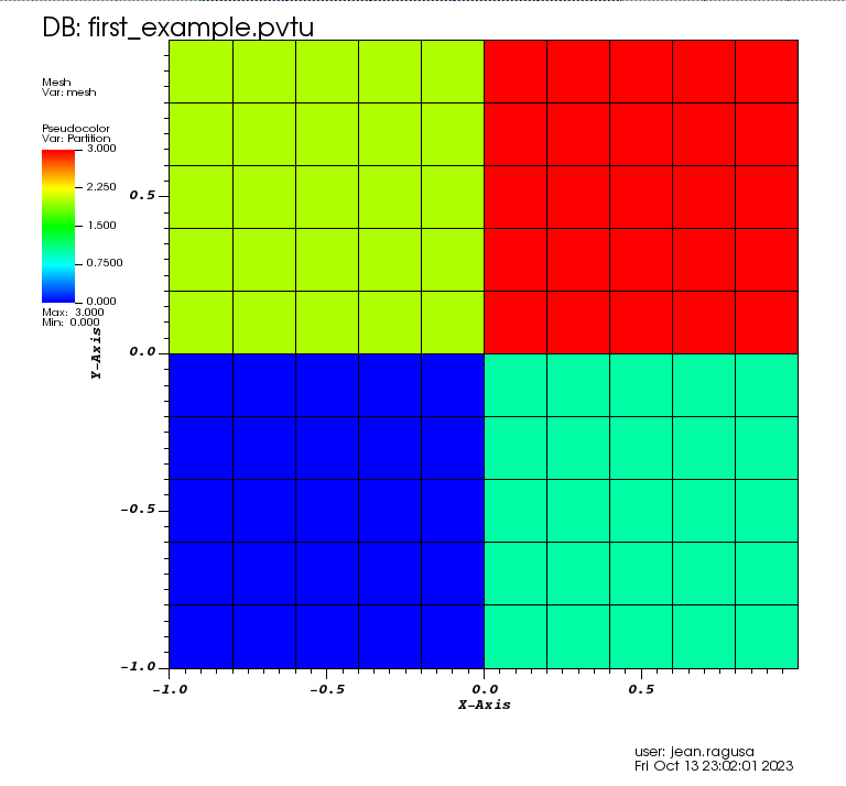
We also partition the 2D mesh into \(2 \times 2\) subdomains using KBAGraphPartitioner. Since we want the split the x-axis in 2, we give only 1 value in the xcuts array (\(x=0\)). Likewise for ycuts (\(y=0\)). The assignment to a partition is done based on where the cell center is located with respect to the various xcuts, ycuts, and zcuts (in the code, a fuzzy logic is applied to avoid arithmetic issues).

The resulting mesh and partition is shown below:

meshgen = OrthogonalMeshGenerator(
    node_sets=[nodes, nodes],
    partitioner=KBAGraphPartitioner(
        nx=2,
        ny=2,
        xcuts=[0.0],
        ycuts=[0.0],
    )
)
grid = meshgen.Execute()

4.1.3.3. Material IDs

When using the in-house OrthogonalMeshGenerator, no material IDs are assigned. The user needs to assign material IDs to all cells. Here, we have a homogeneous domain, so we assign a material ID with value 0 for each cell in the spatial domain.

grid.SetUniformBlockID(0)

4.1.4. Cross Sections

We create one-group cross sections using a built-in method. See the tutorials’ section on cross sections for more details on how to load cross sections into OpenSn.

xs_mat = MultiGroupXS()
xs_mat.CreateSimpleOneGroup(sigma_t=1.,c=0.7)

4.1.5. Volumetric Source

We create a volumetric multigroup source which will be assigned to cells with given block IDs. Volumetric sources are assigned to the solver via the options parameter in the LBS block (see below).

num_groups = 1
strength = []
for g in range(num_groups):
    strength.append(1.0)
mg_src = VolumetricSource(block_ids=[0], group_strength=strength)

4.1.6. Angular Quadrature

We create a product Gauss-Legendre-Chebyshev angular quadrature and pass the total number of polar cosines (here npolar = 4) and the number of azimuthal subdivisions in four quadrants (nazimu = 4). This creates a 2D angular quadrature for XY geometry.

nazimu = 4
npolar = 2
pquad = GLCProductQuadrature2DXY(npolar, nazimu)

4.1.7. Linear Boltzmann Solver

4.1.7.1. Options for the Linear Boltzmann Problem (LBS)

In the LBS block, we provide

• the number of energy groups,

• the groupsets (with 0-indexing), the handle for the angular quadrature, the angle aggregation, the solver type, tolerances, and other solver options.

phys = DiscreteOrdinatesProblem(
    mesh=grid,
    num_groups=num_groups,
    groupsets=[
        {
            "groups_from_to": (0, 0),
            "angular_quadrature": pquad,
            "angle_aggregation_num_subsets": 1,
            "inner_linear_method": "petsc_gmres",
            "l_abs_tol": 1.0e-6,
            "l_max_its": 300,
            "gmres_restart_interval": 30
        }
    ],
    options={
        "volumetric_sources": [mg_src],
    },
    xs_map=[
        {
            "block_ids": [0],
            "xs": xs_mat
        }
    ]
)

4.1.7.2. Putting the Linear Boltzmann Solver Together

We then create the physics solver, initialize it, and execute it.

ss_solver = SteadyStateSolver(lbs_problem=phys)
ss_solver.Initialize()
ss_solver.Execute()

4.1.8. Post-Processing via Field Functions

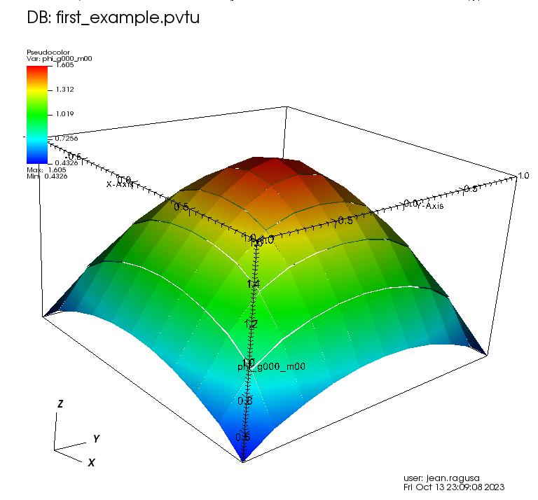
We extract the scalar flux (i.e., the first entry in the field function list; recall that lua indexing starts at 1) and export it to a VTK file whose name is supplied by the user. See the tutorials’ section on post-processing for more details on field functions.

The resulting scalar flux is shown below:

fflist = phys.GetScalarFieldFunctionList(only_scalar_flux=False)
vtk_basename = "first_example"
FieldFunctionGridBased.ExportMultipleToVTK(
    [fflist[0][0]],  # export only the flux of group 0 (first []), moment 0 (second [])
    vtk_basename
)

4.1.9. Finalize (for Jupyter Notebook only)

In Python script mode, PyOpenSn automatically handles environment termination. However, this automatic finalization does not occur when running in a Jupyter notebook, so explicit finalization of the environment at the end of the notebook is required. Do not call the finalization in Python script mode, or in console mode.

Note that PyOpenSn’s finalization must be called before MPI’s finalization.

from IPython import get_ipython

def finalize_env():
    Finalize()
    MPI.Finalize()

ipython_instance = get_ipython()
if ipython_instance is not None:
    ipython_instance.events.register("post_execute", finalize_env)

4.1.10. Possible Extensions

1. Change the number of MPI processes;

2. Change the spatial resolution by increasing or decreasing the number of cells;

3. Change the angular resolution by increasing or decreasing the number of polar and azimuthal subdivisions.