4.2. Slowing-Down in High-Density Polyethylene
[ ]:
import os
import sys
import numpy as np
4.2.1. Using this Notebook
Before running this example, make sure that the Python module of OpenSn was installed.
4.2.1.1. Converting and Running this Notebook from the Terminal
To run this notebook from the terminal, simply type:
jupyter nbconvert --to python --execute <notebook_name>.ipynb.
To run this notebook in parallel (for example, using 4 processes), simply type:
mpiexec -n 4 jupyter nbconvert --to python --execute <notebook_name>.ipynb.
[ ]:
from mpi4py import MPI
size = MPI.COMM_WORLD.size
rank = MPI.COMM_WORLD.rank

if rank == 0:
    print(f"Running with {size} MPI processors.")
4.2.2. Import Requirements
Import required classes and functions from the Python interface of OpenSn. Make sure that the path to PyOpenSn is appended to Python’s PATH.
[ ]:
# assuming that the execute dir is the notebook dir
# this line is not necessary when PyOpenSn is installed using pip
sys.path.append("../../..")

from pyopensn.mesh import OrthogonalMeshGenerator
from pyopensn.xs import MultiGroupXS
from pyopensn.source import VolumetricSource
from pyopensn.aquad import GLCProductQuadrature2DXY
from pyopensn.solver import DiscreteOrdinatesProblem, SteadyStateSourceSolver
from pyopensn.fieldfunc import FieldFunctionGridBased, FieldFunctionInterpolationVolume
from pyopensn.logvol import RPPLogicalVolume

from pyopensn.context import UseColor, Finalize
4.2.2.1. Disable colorized output
[ ]:
UseColor(False)
4.2.3. Mesh
Here, we use the in-house orthogonal mesh generator for a simple Cartesian grid.
We first create a list of nodes for each dimension (X and Y). Here, both dimensions share the same node values.
The nodes will be spread from -10 to +10.
[ ]:
nodes = []
n_cells = 10
length = 20.0
xmin = - length / 2
dx = length / n_cells
for i in range(n_cells + 1):
    nodes.append(xmin + i * dx)
[ ]:
meshgen = OrthogonalMeshGenerator(
    node_sets=[nodes, nodes])
grid = meshgen.Execute()
4.2.3.1. Material IDs
When using the in-house OrthogonalMeshGenerator, no material IDs are assigned. We assign a material ID with value 0 for each cell in the spatial domain.
[ ]:
grid.SetUniformBlockID(0)
4.2.4. Cross Sections
We load 172-group cross sections that were generated using OpenMC.
[ ]:
xs_mat = MultiGroupXS()
xs_mat.LoadFromOpenMC("./HDPE.h5", "set1", 294.0)
num_groups = xs_mat.num_groups
4.2.5. Volumetric Source
We create a volumetric multigroup source which will be assigned to cells with given block IDs. Volumetric sources are assigned to the solver via the options parameter in the LBS block (see below).
[ ]:
strength = np.ones(num_groups)
mg_src = VolumetricSource(block_ids=[0], group_strength=list(strength))
4.2.6. Angular Quadrature
We create a product Gauss-Legendre-Chebyshev angular quadrature and pass the total number of polar cosines (here n_polar = 2) and the number of azimuthal subdivisions in four quadrants (n_azimuthal = 4). This creates a 2D angular quadrature for XY geometry.
[ ]:
pquad = GLCProductQuadrature2DXY(n_polar=2, n_azimuthal=4, scattering_order=0)
4.2.7. Linear Boltzmann Solver
4.2.7.1. Options for the Linear Boltzmann Problem (LBS)
In the LBS block, we provide
the number of energy groups,
the groupsets (with 0-indexing), the handle for the angular quadrature, the angle aggregation, the solver type, tolerances, and other solver options.
[ ]:
phys = DiscreteOrdinatesProblem(
    mesh=grid,
    num_groups=num_groups,
    groupsets=[
        {
            "groups_from_to": (0, num_groups-1),
            "angular_quadrature": pquad,
            "angle_aggregation_num_subsets": 1,
            "inner_linear_method": "petsc_gmres",
            "l_abs_tol": 1.0e-6,
            "l_max_its": 300,
            "gmres_restart_interval": 30
        }
    ],
    scattering_order=0,
    volumetric_sources=[mg_src],
    xs_map=[
        {
            "block_ids": [0],
            "xs": xs_mat
        }
    ]
)
4.2.7.2. Putting the Linear Boltzmann Solver Together
We then create the physics solver, initialize it, and execute it.
[ ]:
ss_solver = SteadyStateSourceSolver(problem=phys)
ss_solver.Initialize()
ss_solver.Execute()
4.2.8. Post-Processing via Field Functions
[ ]:
fflist = phys.GetScalarFieldFunctionList(only_scalar_flux=True)
vtk_basename = "hdpe_ex"
FieldFunctionGridBased.ExportMultipleToPVTU([fflist[g] for g in range(num_groups)], vtk_basename)
4.2.9. Post-processing: Extract the average flux in a portion of the domain
We create an edit zone (logical volume) that is the entire domain.
We request the average (keyword "avg") of the scalar flux over the edit zone, for each group.
[ ]:
logvol_whole_domain = RPPLogicalVolume(infx=True, infy=True, infz=True)
[ ]:
flux = np.zeros(num_groups)
for g in range(0, num_groups):
    ffi = FieldFunctionInterpolationVolume()
    ffi.SetOperationType("sum")
    ffi.SetLogicalVolume(logvol_whole_domain)
    ffi.AddFieldFunction(fflist[g])
    ffi.Initialize()
    ffi.Execute()
    flux[g] = ffi.GetValue()

flux /= np.sum(flux)
[ ]:
# 172-group structure (copied from openmc/openmc/mgxs/__init__.py)
group_edges = np.array([
    1.00001e-05, 3.00000e-03, 5.00000e-03, 6.90000e-03, 1.00000e-02,
    1.50000e-02, 2.00000e-02, 2.50000e-02, 3.00000e-02, 3.50000e-02,
    4.20000e-02, 5.00000e-02, 5.80000e-02, 6.70000e-02, 7.70000e-02,
    8.00000e-02, 9.50000e-02, 1.00001e-01, 1.15000e-01, 1.34000e-01,
    1.40000e-01, 1.60000e-01, 1.80000e-01, 1.89000e-01, 2.20000e-01,
    2.48000e-01, 2.80000e-01, 3.00000e-01, 3.14500e-01, 3.20000e-01,
    3.50000e-01, 3.91000e-01, 4.00000e-01, 4.33000e-01, 4.85000e-01,
    5.00000e-01, 5.40000e-01, 6.25000e-01, 7.05000e-01, 7.80000e-01,
    7.90000e-01, 8.50000e-01, 8.60000e-01, 9.10000e-01, 9.30000e-01,
    9.50000e-01, 9.72000e-01, 9.86000e-01, 9.96000e-01, 1.02000e+00,
    1.03500e+00, 1.04500e+00, 1.07100e+00, 1.09700e+00, 1.11000e+00,
    1.12535e+00, 1.15000e+00, 1.17000e+00, 1.23500e+00, 1.30000e+00,
    1.33750e+00, 1.37000e+00, 1.44498e+00, 1.47500e+00, 1.50000e+00,
    1.59000e+00, 1.67000e+00, 1.75500e+00, 1.84000e+00, 1.93000e+00,
    2.02000e+00, 2.10000e+00, 2.13000e+00, 2.36000e+00, 2.55000e+00,
    2.60000e+00, 2.72000e+00, 2.76792e+00, 3.30000e+00, 3.38075e+00,
    4.00000e+00, 4.12925e+00, 5.04348e+00, 5.34643e+00, 6.16012e+00,
    7.52398e+00, 8.31529e+00, 9.18981e+00, 9.90555e+00, 1.12245e+01,
    1.37096e+01, 1.59283e+01, 1.94548e+01, 2.26033e+01, 2.49805e+01,
    2.76077e+01, 3.05113e+01, 3.37201e+01, 3.72665e+01, 4.01690e+01,
    4.55174e+01, 4.82516e+01, 5.15780e+01, 5.55951e+01, 6.79041e+01,
    7.56736e+01, 9.16609e+01, 1.36742e+02, 1.48625e+02, 2.03995e+02,
    3.04325e+02, 3.71703e+02, 4.53999e+02, 6.77287e+02, 7.48518e+02,
    9.14242e+02, 1.01039e+03, 1.23410e+03, 1.43382e+03, 1.50733e+03,
    2.03468e+03, 2.24867e+03, 3.35463e+03, 3.52662e+03, 5.00451e+03,
    5.53084e+03, 7.46586e+03, 9.11882e+03, 1.11378e+04, 1.50344e+04,
    1.66156e+04, 2.47875e+04, 2.73944e+04, 2.92830e+04, 3.69786e+04,
    4.08677e+04, 5.51656e+04, 6.73795e+04, 8.22975e+04, 1.11090e+05,
    1.22773e+05, 1.83156e+05, 2.47235e+05, 2.73237e+05, 3.01974e+05,
    4.07622e+05, 4.50492e+05, 4.97871e+05, 5.50232e+05, 6.08101e+05,
    8.20850e+05, 9.07180e+05, 1.00259e+06, 1.10803e+06, 1.22456e+06,
    1.35335e+06, 1.65299e+06, 2.01897e+06, 2.23130e+06, 2.46597e+06,
    3.01194e+06, 3.67879e+06, 4.49329e+06, 5.48812e+06, 6.06531e+06,
    6.70320e+06, 8.18731e+06, 1.00000e+07, 1.16183e+07, 1.38403e+07,
    1.49182e+07, 1.73325e+07, 1.96403e+07])

# flip group edges to have highest energies first, since fastest groups have the lowest index
E = np.flip(group_edges)
# compute the group widths
dE = -np.diff(E)
# compute the group midpoints
Emid = E[:-1] + dE/2
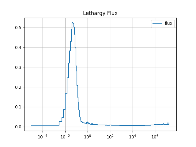
[ ]:
import matplotlib.pyplot as plt
plt.figure()
y = Emid * flux / dE
y = np.insert(y, 0, y[0])
plt.semilogx(E, y, drawstyle='steps',label='flux')
plt.title('Lethargy Flux')
plt.legend()
plt.grid()
# plt.savefig("images/hdpe_example_lethargy_spectrum.png")
plt.show()
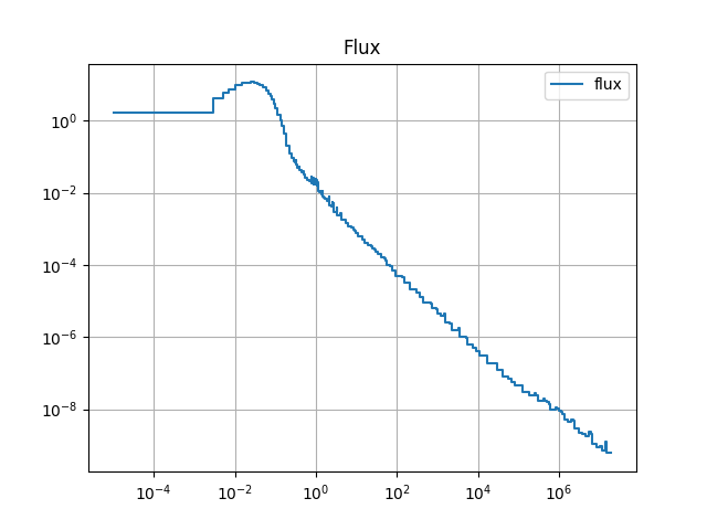
plt.figure()
y = flux / dE
y = np.insert(y, 0, y[0])
plt.loglog(E, y, drawstyle='steps',label='flux')
plt.title('Flux')
plt.legend()
plt.grid()
# plt.savefig("images/hdpe_example_spectrum.png")
plt.show()
The resulting spectra are shown below:
4.2.10. Finalize (for Jupyter Notebook only)
In Python script mode, PyOpenSn automatically handles environment termination. However, this automatic finalization does not occur when running in a Jupyter notebook, so explicit finalization of the environment at the end of the notebook is required. Do not call the finalization in Python script mode, or in console mode.
Note that PyOpenSn’s finalization must be called before MPI’s finalization.
[ ]:
from IPython import get_ipython

def finalize_env():
    Finalize()
    MPI.Finalize()

ipython_instance = get_ipython()
if ipython_instance is not None:
    ipython_instance.events.register("post_execute", finalize_env)