2.6.5. Arbitrary Angular Boundary Source

This tutorial imports a Gmsh mesh whose physical groups identify a boundary-source segment and uses an AngularFluxFunction to illuminate that segment only along directions inside a cone about the inward \(+x\) direction.

2.6.5.1. Build the mesh

The imported Gmsh mesh covers the unit square. Its two-dimensional Background physical group has block ID 1, while one-dimensional physical groups name the exterior boundaries. The centered segment \(0.4 \leq y \leq 0.6\) on the left edge is named Boundary_Source; the rest of that edge is xmin. Because OpenSn imports these physical groups as boundary IDs, no logical volume or call to SetOrthogonalBoundaries is needed.

from mpi4py import MPI
from pyopensn.aquad import GLCProductQuadrature2DXY
from pyopensn.context import Finalize
from pyopensn.math import AngularFluxFunction
from pyopensn.mesh import FromFileMeshGenerator, PETScGraphPartitioner
from pyopensn.solver import DiscreteOrdinatesProblem, SteadyStateSourceSolver
from pyopensn.xs import MultiGroupXS

rank = MPI.COMM_WORLD.rank
mesh = FromFileMeshGenerator(
    filename="Square.msh",
    partitioner=PETScGraphPartitioner(type="parmetis"),
).Execute()

xs = MultiGroupXS()
xs.CreateSimpleOneGroup(sigma_t=1.0, c=0.8)
quadrature = GLCProductQuadrature2DXY(
    n_polar=2, n_azimuthal=128, scattering_order=0
)
groupset = {
    "groups_from_to": (0, 0),
    "angular_quadrature": quadrature,
    "inner_linear_method": "petsc_gmres",
    "l_abs_tol": 1.0e-10,
    "l_max_its": 500,
}

2.6.5.2. Define the angular boundary source

For a direction \(\boldsymbol{\Omega}\), its cosine relative to the \(+x\) axis is \(\Omega_x = \cos(\theta)\). The cone contains directions satisfying \(\Omega_x \geq 0.8\), corresponding to a half-angle of \(\cos^{-1}(0.8) \approx 0.644\) radians. The callback returns an incoming angular flux of 0.5 for those directions in group 0 and zero otherwise.

The callback receives indices rather than an angle object, so the direction mask is built from the same quadrature assigned to the groupset. The callback is uniform over a named boundary, and the imported Boundary_Source physical group restricts it to the desired spatial segment.

cone_cosine_cutoff = 0.8
selected_directions = {
    direction_index
    for direction_index, omega in enumerate(quadrature.omegas)
    if omega.x >= cone_cosine_cutoff
}
if not selected_directions:
    raise RuntimeError("The angular quadrature has no directions inside the cone.")

def xmin_bc_func(group_index, direction_index):
    if group_index == 0 and direction_index in selected_directions:
        return 0.5
    return 0.0

xmin_bc = AngularFluxFunction(xmin_bc_func)
boundary_conditions = [
    {"name": "Boundary_Source", "type": "arbitrary", "function": xmin_bc},
    {"name": "xmin", "type": "vacuum"},
    {"name": "xmax", "type": "vacuum"},
    {"name": "ymin", "type": "vacuum"},
    {"name": "ymax", "type": "vacuum"},
]

2.6.5.3. Configure and solve the problem

The arbitrary boundary is passed through the same boundary-condition list used for built-in isotropic, vacuum, and reflecting conditions. Angular-flux storage and balance accounting support the leakage and conservation checks below.

problem = DiscreteOrdinatesProblem(
    mesh=mesh,
    num_groups=1,
    groupsets=[groupset],
    xs_map=[{"block_ids": [1], "xs": xs}],
    boundary_conditions=boundary_conditions,
    options={"save_angular_flux": True},
)
solver = SteadyStateSourceSolver(problem=problem, compute_balance=True)
solver.Initialize()
solver.Execute()

2.6.5.4. Check the directional source and particle balance

The selected directions must all lie inside the requested cone. Because that cone and the square are symmetric about \(y=0.5\), leakage through ymin and ymax should agree. The balance residual verifies that boundary inflow equals absorption plus total outflow.

leakage = problem.ComputeLeakage(["xmax", "ymin", "ymax"])
transmitted_current = float(leakage["xmax"][0])
lower_leakage = float(leakage["ymin"][0])
upper_leakage = float(leakage["ymax"][0])
symmetry_error = abs(lower_leakage - upper_leakage)

balance = solver.ComputeBalanceTable()
source_rate = balance["production_rate"] + balance["inflow_rate"]
loss_rate = balance["absorption_rate"] + balance["outflow_rate"]
balance_residual = abs(source_rate - loss_rate) / max(abs(source_rate), 1.0e-16)
if rank == 0:
    print(f"Cone direction count={len(selected_directions)}")
    print(f"Arbitrary transmitted current={transmitted_current:.6e}")
    print(f"Arbitrary lower leakage={lower_leakage:.6e}")
    print(f"Arbitrary upper leakage={upper_leakage:.6e}")
    print(f"Arbitrary side symmetry error={symmetry_error:.6e}")
    print(f"Arbitrary balance residual={balance_residual:.6e}")
assert all(
    quadrature.omegas[index].x >= cone_cosine_cutoff
    for index in selected_directions
)
assert transmitted_current > 0.0
assert symmetry_error < 1.0e-8
assert balance_residual < 1.0e-8
if "opensn_console" not in globals():
    from IPython import get_ipython
    if get_ipython() is not None:
        Finalize()
        MPI.Finalize()

2.6.5.5. Visualize the scalar flux

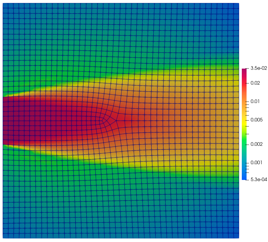
The following optional snippet exports the scalar flux for visualization. It is shown rather than executed so regression tests do not create VTK files.

from pyopensn.fieldfunc import FieldFunctionGridBased

fflist = problem.GetScalarFluxFieldFunction()
FieldFunctionGridBased.ExportMultipleToPVTU(
    [fflist[0]], "Flux/Phi_p"
)

The resulting scalar-flux distribution is shown below.