2.6.4. Isotropic Boundary Source and Leakage

This tutorial sends particles into a two-dimensional, purely absorbing square through an isotropic boundary condition and measures leakage through its three vacuum boundaries.

2.6.4.1. Build the mesh

The square has unit width and height and a unit total cross section with no scattering. A two-dimensional product quadrature resolves directions in the \(x\)-\(y\) plane.

from mpi4py import MPI
from pyopensn.aquad import GLCProductQuadrature2DXY
from pyopensn.context import Finalize
from pyopensn.mesh import OrthogonalMeshGenerator
from pyopensn.solver import DiscreteOrdinatesProblem, SteadyStateSourceSolver
from pyopensn.xs import MultiGroupXS

rank = MPI.COMM_WORLD.rank
num_cells_x = 40
num_cells_y = 40
x_nodes = [i / num_cells_x for i in range(num_cells_x + 1)]
y_nodes = [i / num_cells_y for i in range(num_cells_y + 1)]
mesh = OrthogonalMeshGenerator(node_sets=[x_nodes, y_nodes]).Execute()
mesh.SetUniformBlockID(0)

xs = MultiGroupXS()
xs.CreateSimpleOneGroup(sigma_t=1.0, c=0.0)
quadrature = GLCProductQuadrature2DXY(
    n_polar=2, n_azimuthal=64, scattering_order=0
)
groupset = {
    "groups_from_to": (0, 0),
    "angular_quadrature": quadrature,
    "inner_linear_method": "petsc_gmres",
    "l_abs_tol": 1.0e-10,
    "l_max_its": 100,
}

2.6.4.2. Define the boundary source

The xmin boundary supplies an isotropic group strength of two. The opposite boundary and both horizontal boundaries are vacuum, so particles can be transmitted through xmax or leak through ymin and ymax. Unlike point and volumetric sources, a boundary source is specified directly in the boundary-condition list.

incoming_group_strength = 2.0
boundary_conditions = [
    {
        "name": "xmin",
        "type": "isotropic",
        "group_strength": [incoming_group_strength],
    },
    {"name": "xmax", "type": "vacuum"},
    {"name": "ymin", "type": "vacuum"},
    {"name": "ymax", "type": "vacuum"},
]

2.6.4.3. Configure and solve the problem

Setting save_angular_flux=True retains the directional solution needed to compute leakage. Enabling balance accounting provides an independent check that boundary inflow equals absorption plus total outflow.

problem = DiscreteOrdinatesProblem(
    mesh=mesh,
    num_groups=1,
    groupsets=[groupset],
    xs_map=[{"block_ids": [0], "xs": xs}],
    boundary_conditions=boundary_conditions,
    options={"save_angular_flux": True},
)
solver = SteadyStateSourceSolver(problem=problem, compute_balance=True)
solver.Initialize()
solver.Execute()

2.6.4.4. Check leakage symmetry and particle balance

ComputeLeakage integrates the stored angular flux over each requested boundary. The square, material, source, mesh, and quadrature are symmetric about \(y=0.5\), so leakage through ymin and ymax should agree. The balance residual verifies that inflow is accounted for by absorption and leakage through all three vacuum boundaries.

leakage = problem.ComputeLeakage(["xmax", "ymin", "ymax"])
transmitted_current = float(leakage["xmax"][0])
lower_leakage = float(leakage["ymin"][0])
upper_leakage = float(leakage["ymax"][0])
symmetry_error = abs(lower_leakage - upper_leakage)

balance = solver.ComputeBalanceTable()
source_rate = balance["production_rate"] + balance["inflow_rate"]
loss_rate = balance["absorption_rate"] + balance["outflow_rate"]
balance_residual = abs(source_rate - loss_rate) / max(abs(source_rate), 1.0e-16)
if rank == 0:
    print(f"Transmitted current={transmitted_current:.6e}")
    print(f"Lower leakage={lower_leakage:.6e}")
    print(f"Upper leakage={upper_leakage:.6e}")
    print(f"Side-leakage symmetry error={symmetry_error:.6e}")
    print(f"Balance residual={balance_residual:.6e}")
assert transmitted_current > 0.0
assert symmetry_error < 1.0e-10
assert balance_residual < 1.0e-8
if "opensn_console" not in globals():
    from IPython import get_ipython
    if get_ipython() is not None:
        Finalize()
        MPI.Finalize()

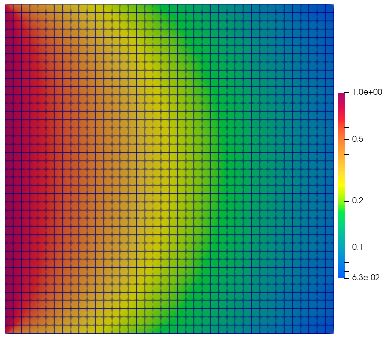
2.6.4.5. Visualize the scalar flux

The following optional snippet exports the scalar flux for visualization. It is shown rather than executed so regression tests do not create VTK files.

from pyopensn.fieldfunc import FieldFunctionGridBased

fflist = problem.GetScalarFluxFieldFunction()
FieldFunctionGridBased.ExportMultipleToPVTU(
    [fflist[0]], "Flux/Phi_p"
)

The resulting scalar-flux distribution is shown below.