4.4.2. Reuse an Uncollided Flux in a Collided Solve
This tutorial builds on Generate and Validate an Uncollided Flux. It reads the saved angular-flux moments, solves for the collided contribution, and compares the total scalar flux with the uncollided scalar flux along the same line.
4.4.2.1. Prerequisite
Run the uncollided-flux tutorial first. It creates uncollided.h5, which supplies the first-collision source, and the line data used below.
[ ]:
import csv
import math
import sys
from pathlib import Path

from mpi4py import MPI

rank = MPI.COMM_WORLD.rank
4.4.2.2. Import OpenSn
[ ]:
repo_root = Path.cwd().resolve()
while repo_root != repo_root.parent and not (repo_root / "test" / "assets").is_dir():
    repo_root = repo_root.parent
if not (repo_root / "test" / "assets").is_dir():
    raise RuntimeError("Could not locate the OpenSn repository root.")

tutorial_dir = repo_root / "doc/source/tutorials/workflows/data_reuse/uncollided"
sys.path.append(str(repo_root / "build"))

from pyopensn.aquad import GLCProductQuadrature3DXYZ
from pyopensn.fieldfunc import (
    FieldFunctionInterpolationLine,
    FieldFunctionInterpolationPoint,
    FieldFunctionInterpolationVolume,
)
from pyopensn.logvol import RPPLogicalVolume
from pyopensn.math import Vector3
from pyopensn.mesh import FromFileMeshGenerator
from pyopensn.solver import DiscreteOrdinatesProblem, SteadyStateSourceSolver
from pyopensn.xs import MultiGroupXS
4.4.2.3. Recover the Saved Data
Both tutorials use the same 5,880-cell mesh, material, and source definitions. The material parameters \(\Sigma_t=40\ \mathrm{m}^{-1}\) and \(c=0.9\) make the cube 1.28 mean-free-paths thick and favor scattering, so the reused first-collision source produces a substantial collided contribution. The uncollided HDF5 data must be generated on exactly the same mesh used by this collided solve. Matching line-sampling points then allow the uncollided and total fluxes to be compared directly.
[ ]:
mesh_file = repo_root / "test/assets/mesh/cube3.2.msh"
uncollided_file = tutorial_dir / "uncollided.h5"
source_location = (0.0102586, 0.0114131, 0.0146416)
sample_point = (0.024, 0.016, 0.008)
sigma_t = 40.0
scattering_ratio = 0.9
num_polar_angles = 4
num_azimuthal_angles = 32

def make_mesh():
    grid = FromFileMeshGenerator(filename=str(mesh_file)).Execute()
    grid.SetUniformBlockID(0)
    return grid

def make_xs():
    xs = MultiGroupXS()
    xs.CreateSimpleOneGroup(sigma_t=sigma_t, c=scattering_ratio)
    return xs

def make_whole_domain():
    return RPPLogicalVolume(
        xmin=-0.001, xmax=0.033,
        ymin=-0.001, ymax=0.033,
        zmin=-0.001, zmax=0.033,
    )

output_dir = tutorial_dir / "tutorial_output"
uncollided_line_file = next(output_dir.glob("uncollided_line_*.csv"), None)
total_line_base = output_dir / "total_line"
line_y = 0.024
line_z = 0.024
line_start = Vector3(0.0, line_y, line_z)
line_end = Vector3(0.032, line_y, line_z)

for required_file in (uncollided_file, uncollided_line_file):
    if required_file is None or not required_file.exists():
        raise RuntimeError(
            f"Missing {required_file}. Run uncollided.ipynb before this tutorial."
        )

def point_value(field_function, point):
    interpolation = FieldFunctionInterpolationPoint()
    interpolation.SetPointOfInterest(Vector3(*point))
    interpolation.AddFieldFunction(field_function)
    interpolation.Execute()
    return interpolation.GetPointValue()

def volume_integral(field_function, logical_volume):
    interpolation = FieldFunctionInterpolationVolume()
    interpolation.SetOperationType("sum")
    interpolation.SetLogicalVolume(logical_volume)
    interpolation.AddFieldFunction(field_function)
    interpolation.Execute()
    return interpolation.GetValue()

def read_line_data(csv_file):
    with csv_file.open(newline="") as stream:
        rows = list(csv.DictReader(stream))
    data = sorted(
        ((float(row["x"]), float(row["phi_g000_m00"])) for row in rows),
        key=lambda item: item[0],
    )
    return [p[0] for p in data], [p[1] for p in data]

def export_line_data(field_function, base_name):
    for old_file in base_name.parent.glob(f"{base_name.name}*.csv"):
        old_file.unlink()
    interpolation = FieldFunctionInterpolationLine()
    interpolation.SetInitialPoint(line_start)
    interpolation.SetFinalPoint(line_end)
    interpolation.SetNumberOfPoints(200)
    interpolation.AddFieldFunction(field_function)
    interpolation.Execute()
    interpolation.ExportToCSV(str(base_name))
    return read_line_data(next(base_name.parent.glob(f"{base_name.name}_*.csv")))
4.4.2.4. Solve the Collided Problem
Passing the HDF5 file through uncollided_flux constructs the first-collision source from the saved moments. The collided calculation uses four polar and 32 azimuthal angles, for 128 discrete directions. The uncollided stage itself is ray traced and therefore does not use this angular quadrature. The returned scalar flux is the total,
where \(\phi_u\) and \(\phi_c\) are the uncollided and collided contributions.
[ ]:
grid = make_mesh()
xs = make_xs()
whole_domain = make_whole_domain()

quadrature = GLCProductQuadrature3DXYZ(
    n_polar=num_polar_angles,
    n_azimuthal=num_azimuthal_angles,
    scattering_order=0,
)
problem = DiscreteOrdinatesProblem(
    mesh=grid,
    num_groups=1,
    groupsets=[{
        "groups_from_to": [0, 0],
        "angular_quadrature": quadrature,
        "angle_aggregation_type": "single",
        "inner_linear_method": "petsc_gmres",
        "gmres_restart_interval": 30,
        "l_abs_tol": 1.0e-8,
        "l_max_its": 200,
    }],
    xs_map=[{"block_ids": [0], "xs": xs}],
    uncollided_flux=str(uncollided_file),
)
solver = SteadyStateSourceSolver(problem=problem, compute_balance=True)
solver.Initialize()
solver.Execute()
4.4.2.5. Post-Process the Total Flux
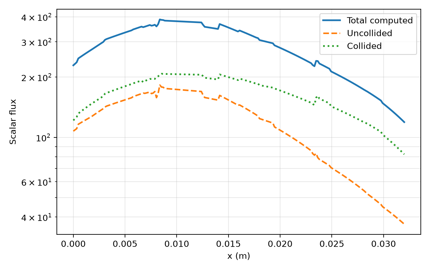
The point and volume metrics are retained for regression testing. A second line interpolation supplies the total flux for comparison with the saved uncollided values. We also report the collided fraction of the line-integrated total to quantify the effect of scattering.
[ ]:
scalar_flux = problem.GetScalarFluxFieldFunction()[0]
point_flux = point_value(scalar_flux, sample_point)
total_integral = volume_integral(scalar_flux, whole_domain)
balance = solver.ComputeBalanceTable()["balance"]

line_x, line_total = export_line_data(scalar_flux, total_line_base)
uncollided_x, line_uncollided = read_line_data(uncollided_line_file)
if len(line_x) != len(uncollided_x) or any(
    not math.isclose(a, b, abs_tol=1.0e-12)
    for a, b in zip(line_x, uncollided_x)
):
    raise RuntimeError("The total and uncollided sampling points do not match.")

line_collided = [
    total - uncollided
    for total, uncollided in zip(line_total, line_uncollided)
]
collided_line_fraction = sum(line_collided) / sum(line_total)

if rank == 0:
    print(f"Total scalar flux at {sample_point}: {point_flux:.12e}")
    print(f"Total scalar-flux integral: {total_integral:.12e}")
    print(f"Balance residual: {balance:.12e}")
    print(f"Maximum collided line flux: {max(line_collided):.12e}")
    print(f"Collided fraction of line-integrated flux: {collided_line_fraction:.12e}")
assert 0.5 < collided_line_fraction < 1.0
4.4.2.6. Compare the Total and Uncollided Fluxes
Subtracting the saved uncollided line values from the total isolates the collided contribution. For this moderately thick, strongly scattering material, the collided flux supplies about 60% of the line-integrated total and visibly separates the total curve from the uncollided curve. The curves retain the cell-boundary jumps of the sweep-based PWLD spatial solution; these are discretization effects on the 5,880-cell mesh and should decrease under mesh refinement.
[ ]:
import matplotlib.pyplot as plt

fig, ax = plt.subplots(figsize=(7.0, 4.4))
ax.semilogy(line_x, line_total, "-", lw=2.0, label="Total computed")
ax.semilogy(line_x, line_uncollided, "--", lw=1.8, label="Uncollided")
ax.semilogy(line_x, line_collided, ":", lw=2.0, label="Collided")
ax.set_xlabel("x (m)")
ax.set_ylabel("Scalar flux")
ax.grid(True, which="both", alpha=0.3)
ax.legend()
fig.tight_layout()

# The documentation uses the saved image below. Uncomment only to regenerate it.
# fig.savefig(tutorial_dir / "images/collided_flux_comparison.png", dpi=200)

fig