4.4.1. Generate and Validate an Uncollided Flux

This tutorial computes the uncollided angular-flux moments from an isotropic point source in a homogeneous three-dimensional cube containing 5,880 tetrahedral cells. The result is written to uncollided.h5 for reuse by the collided-flux tutorial.

The scalar flux is also compared with the analytic uncollided solution along a line offset from the source. Avoiding the point-source singularity makes this a meaningful comparison.

4.4.1.1. Prerequisites

This example runs in serial and requires the OpenSn Python module.

import csv
import math
import sys
from pathlib import Path

from mpi4py import MPI

rank = MPI.COMM_WORLD.rank
size = MPI.COMM_WORLD.size
if size != 1:
    raise RuntimeError("The uncollided-flux file must be generated in serial.")

4.4.1.2. Import OpenSn

Locate the repository root so the notebook works both interactively and through the documentation regression-test driver.

repo_root = Path.cwd().resolve()
while repo_root != repo_root.parent and not (repo_root / "test" / "assets").is_dir():
    repo_root = repo_root.parent
if not (repo_root / "test" / "assets").is_dir():
    raise RuntimeError("Could not locate the OpenSn repository root.")

tutorial_dir = repo_root / "doc/source/tutorials/workflows/data_reuse/uncollided"
sys.path.append(str(repo_root / "build"))

from pyopensn.fieldfunc import FieldFunctionInterpolationLine, FieldFunctionInterpolationPoint
from pyopensn.logvol import RPPLogicalVolume
from pyopensn.math import Vector3
from pyopensn.mesh import FromFileMeshGenerator
from pyopensn.solver import UncollidedProblem, UncollidedSolver
from pyopensn.source import PointSource
from pyopensn.xs import MultiGroupXS

4.4.1.3. Define the Line-Sampling Utilities

Both tutorials use the same mesh, material, source, and domain definitions. The cube3.2.msh mesh discretizes the 3.2-cm cube into 5,880 tetrahedral cells. The material has \(\Sigma_t=40\ \mathrm{m}^{-1}\) and scattering ratio \(c=0.9\), giving an optical thickness of 1.28. This makes collisions common while directing 90% of interactions into scattering. The validation line is offset from the source so every analytic value is finite and spatially resolved.

mesh_file = repo_root / "test/assets/mesh/cube3.2.msh"
uncollided_file = tutorial_dir / "uncollided.h5"
source_location = (0.0102586, 0.0114131, 0.0146416)
sample_point = (0.024, 0.016, 0.008)
sigma_t = 40.0
scattering_ratio = 0.9

def make_mesh():
    grid = FromFileMeshGenerator(filename=str(mesh_file)).Execute()
    grid.SetUniformBlockID(0)
    return grid

def make_xs():
    xs = MultiGroupXS()
    xs.CreateSimpleOneGroup(sigma_t=sigma_t, c=scattering_ratio)
    return xs

def make_near_source_region():
    width = 0.008
    return RPPLogicalVolume(
        xmin=source_location[0] - width, xmax=source_location[0] + width,
        ymin=source_location[1] - width, ymax=source_location[1] + width,
        zmin=source_location[2] - width, zmax=source_location[2] + width,
    )

output_dir = tutorial_dir / "tutorial_output"
output_dir.mkdir(exist_ok=True)
line_y = 0.024
line_z = 0.024
line_start = Vector3(0.0, line_y, line_z)
line_end = Vector3(0.032, line_y, line_z)
line_base = output_dir / "uncollided_line"

def point_value(field_function, point):
    interpolation = FieldFunctionInterpolationPoint()
    interpolation.SetPointOfInterest(Vector3(*point))
    interpolation.AddFieldFunction(field_function)
    interpolation.Execute()
    return interpolation.GetPointValue()

def export_line_data(field_function, base_name, start=None, end=None):
    for old_file in base_name.parent.glob(f"{base_name.name}*.csv"):
        old_file.unlink()
    interpolation = FieldFunctionInterpolationLine()
    interpolation.SetInitialPoint(start if start is not None else line_start)
    interpolation.SetFinalPoint(end if end is not None else line_end)
    interpolation.SetNumberOfPoints(200)
    interpolation.AddFieldFunction(field_function)
    interpolation.Execute()
    interpolation.ExportToCSV(str(base_name))
    csv_file = next(base_name.parent.glob(f"{base_name.name}_*.csv"))
    with csv_file.open(newline="") as stream:
        rows = list(csv.DictReader(stream))
    data = sorted(
        ((float(row["x"]), float(row["phi_g000_m00"])) for row in rows),
        key=lambda item: item[0],
    )
    return csv_file, [p[0] for p in data], [p[1] for p in data]

def analytic_flux_at(x, y, z):
    radius = math.dist((x, y, z), source_location)
    return math.exp(-sigma_t * radius) / (4.0 * math.pi * radius**2)

def analytic_uncollided_flux(x):
    return analytic_flux_at(x, line_y, line_z)

4.4.1.4. Compute the Uncollided Flux

The uncollided solver writes angular-flux moments to an HDF5 file. The next tutorial reads this file as an external first-collision source.

uncollided_file.unlink(missing_ok=True)
grid = make_mesh()
xs = make_xs()
near_source_region = make_near_source_region()

uncollided_problem = UncollidedProblem(
    mesh=grid,
    num_groups=1,
    groupsets=[{"groups_from_to": [0, 0]}],
    xs_map=[{"block_ids": [0], "xs": xs}],
    point_sources=[
        PointSource(location=list(source_location), strength=[1.0])
    ],
    near_source=[near_source_region],
    scattering_order=0,
)
uncollided_solver = UncollidedSolver(
    problem=uncollided_problem,
    file_name=str(uncollided_file),
    progress_interval=25,
)
uncollided_solver.Initialize()
uncollided_solver.Execute()

4.4.1.5. Compare with the Analytic Solution

For a unit-strength isotropic point source in a homogeneous medium,

\[\phi_u(r)=\frac{\exp(-\Sigma_t r)}{4\pi r^2}.\]

Because the line is offset from the point source, all sampled locations are included in the error calculation. The line data are retained for the collided tutorial.

uncollided_flux = uncollided_problem.GetScalarFluxFieldFunction()[0]
line_csv, line_x, line_uncollided = export_line_data(uncollided_flux, line_base)

comparison = [
    (x, value, analytic_uncollided_flux(x))
    for x, value in zip(line_x, line_uncollided)
]
relative_errors = [
    abs(numerical - analytic) / analytic
    for _, numerical, analytic in comparison
]
sample_numerical = point_value(uncollided_flux, sample_point)
sample_radius = math.dist(sample_point, source_location)
sample_analytic = math.exp(-sigma_t * sample_radius) / (
    4.0 * math.pi * sample_radius**2
)
sample_relative_error = abs(sample_numerical - sample_analytic) / sample_analytic
line_mean_relative_error = sum(relative_errors) / len(relative_errors)
if line_mean_relative_error > 0.03 or sample_relative_error > 0.08:
    raise RuntimeError("Uncollided flux does not agree with the analytic solution.")

if rank == 0:
    print(f"UncollidedFile={uncollided_file}")
    print(f"UncollidedLineFile={line_csv}")
    print(f"AnalyticComparisonPoints={len(comparison)}")
    print(f"UncollidedLineMeanRelativeError={line_mean_relative_error:.12e}")
    print(f"UncollidedLineMaxRelativeError={max(relative_errors):.12e}")
    print(f"UncollidedSampleOpenSn={sample_numerical:.12e}")
    print(f"UncollidedSampleAnalytic={sample_analytic:.12e}")
    print(f"UncollidedSampleRelativeError={sample_relative_error:.12e}")

4.4.1.6. Visualize the Uncollided Flux

The small near-source region is ray traced, while the remaining cells exercise the sweep-based bulk algorithm. The line plot shows the OpenSn and analytic values at every sampled location. The line is offset from the source by \(\sqrt{0.0126^2+0.00936^2}\approx 0.0157\) m, so it retains a smooth peak centered near \(x=0.0103\) m without intersecting the singularity.

The plot uses 200 samples on the same 5,880-cell mesh used throughout the tutorial. The validation line lies entirely outside the ray-traced near-source region: its offsets of about 0.0126 m in y and 0.00936 m in z both exceed the region’s 0.008 m half-width, so every sampled value comes from the sweep-based bulk solve. The jumps in the OpenSn curve occur where the line crosses tetrahedral-cell boundaries within that sweep-based region. They are a visible spatial-discretization effect of the sweep-based PWLD solution, rather than random noise or reduced plotting resolution, and decrease under mesh refinement, confirmed quantitatively below.

import matplotlib.pyplot as plt

plot_x = line_x
plot_numerical = line_uncollided
plot_analytic = [analytic_uncollided_flux(x) for x in line_x]

fig, ax = plt.subplots(figsize=(7.0, 4.4))
ax.semilogy(
    plot_x, plot_numerical, "--+", ms=5, markevery=4,
    label="OpenSn uncollided",
)
ax.semilogy(
    plot_x, plot_analytic, "--.", ms=5, markevery=4,
    label="Analytic uncollided",
)
ax.set_xlabel("x (m)")
ax.set_ylabel("Scalar flux")
ax.grid(True, which="both", alpha=0.3)
ax.legend()
fig.tight_layout()

# The documentation uses the saved image below. Uncomment only to regenerate it.
# fig.savefig(tutorial_dir / "images/uncollided_flux_comparison.png", dpi=200)

fig

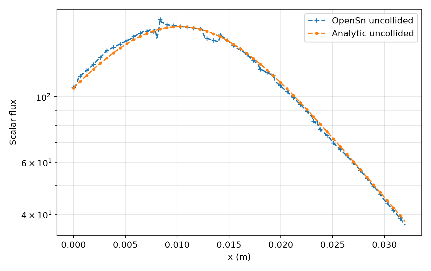
The plot above uses the 5,880-cell cube3.2.msh tetrahedral mesh, a 0.016 m near-source region (0.008 m half-width) evaluated with OpenSn’s fixed fourth-order spatial quadrature, and 200 line samples for both the OpenSn and analytic curves.

The HDF5 and CSV outputs now provide the inputs required by the collided-flux tutorial.

4.4.1.7. Confirm Mesh-Refinement Convergence

The jumps described above are a spatial-discretization effect, so refining the mesh should reduce them. To check this quantitatively rather than only by eye, the same problem is solved again on cube3.2_fine.msh — a second mesh of the same 3.2-cm cube, graded from about 0.6 mm elements near the point source out to 1.8 mm in the bulk, for roughly 46,000 tetrahedral cells.

The refinement is graded rather than uniform on purpose. A uniform refinement does not control how close the point source lands to a cell face, and OpenSn’s point-source representation is measurably sensitive to that: if the source sits close to a face relative to its cell’s size, OpenSn emits a warning (UncollidedProblem: point source ... lies only <dist> from a face of its containing cell) because the near-source ray-traced flux is poorly resolved there. Grading the mesh finer around the source keeps its containing cell small and well-shaped regardless of exactly where the mesh generator places it, so the comparison below isolates the effect of resolution rather than an accident of meshing.

The plots above only show the sweep-based bulk region, since the validation line is offset enough in y and z to stay outside the 0.008 m near-source half-width for every x. To also see the ray-traced region, a second line is sampled here, offset by only 0.006 m in both y and z instead — small enough to pass through the near-source region for \(x\in[0.0023,0.0183]\) m, while its closest approach to the source (0.00849 m, at \(x=x_\mathrm{source}\)) still keeps every analytic value finite. This near-source line reuses the two field functions already solved above; no additional transport solve is needed.

fine_mesh_file = repo_root / "test/assets/mesh/cube3.2_fine.msh"
fine_uncollided_file = output_dir / "uncollided_fine.h5"
fine_uncollided_file.unlink(missing_ok=True)

fine_grid = FromFileMeshGenerator(filename=str(fine_mesh_file)).Execute()
fine_grid.SetUniformBlockID(0)
fine_num_cells = fine_grid.GetGlobalNumberOfCells()

fine_uncollided_problem = UncollidedProblem(
    mesh=fine_grid,
    num_groups=1,
    groupsets=[{"groups_from_to": [0, 0]}],
    xs_map=[{"block_ids": [0], "xs": make_xs()}],
    point_sources=[
        PointSource(location=list(source_location), strength=[1.0])
    ],
    near_source=[make_near_source_region()],
    scattering_order=0,
)
fine_uncollided_solver = UncollidedSolver(
    problem=fine_uncollided_problem,
    file_name=str(fine_uncollided_file),
    progress_interval=25,
)
fine_uncollided_solver.Initialize()
fine_uncollided_solver.Execute()

fine_uncollided_flux = fine_uncollided_problem.GetScalarFluxFieldFunction()[0]
fine_line_csv, fine_line_x, fine_line_uncollided = export_line_data(
    fine_uncollided_flux, output_dir / "uncollided_line_fine"
)

fine_relative_errors = [
    abs(numerical - analytic_uncollided_flux(x)) / analytic_uncollided_flux(x)
    for x, numerical in zip(fine_line_x, fine_line_uncollided)
]
fine_mean_relative_error = sum(fine_relative_errors) / len(fine_relative_errors)
fine_max_relative_error = max(fine_relative_errors)

# The refined mesh must be more accurate than the coarse one -- this is the
# quantitative version of the convergence claim made above -- and both
# errors must stay within sane absolute bounds.
if fine_mean_relative_error >= line_mean_relative_error:
    raise RuntimeError(
        "Refining the mesh did not reduce the mean relative error: "
        f"coarse={line_mean_relative_error:.6e}, fine={fine_mean_relative_error:.6e}"
    )
if fine_mean_relative_error > 0.015 or fine_max_relative_error > 0.05:
    raise RuntimeError("Fine-mesh uncollided flux does not agree with the analytic solution.")

# A second line, offset only 0.006 m in y and z, dips into the ray-traced
# near-source region instead of staying entirely in the swept bulk region.
# Both already-solved field functions are resampled along it -- no new
# transport solve is needed.
near_source_line_y = source_location[1] - 0.006
near_source_line_z = source_location[2] - 0.006
near_source_line_start = Vector3(0.0, near_source_line_y, near_source_line_z)
near_source_line_end = Vector3(0.032, near_source_line_y, near_source_line_z)

_, near_source_line_x, near_source_coarse = export_line_data(
    uncollided_flux, output_dir / "uncollided_near_source_line_coarse",
    start=near_source_line_start, end=near_source_line_end,
)
_, _, near_source_fine = export_line_data(
    fine_uncollided_flux, output_dir / "uncollided_near_source_line_fine",
    start=near_source_line_start, end=near_source_line_end,
)
near_source_analytic = [
    analytic_flux_at(x, near_source_line_y, near_source_line_z) for x in near_source_line_x
]

near_source_coarse_errors = [
    abs(n - a) / a for n, a in zip(near_source_coarse, near_source_analytic)
]
near_source_fine_errors = [
    abs(n - a) / a for n, a in zip(near_source_fine, near_source_analytic)
]
near_source_coarse_mean = sum(near_source_coarse_errors) / len(near_source_coarse_errors)
near_source_fine_mean = sum(near_source_fine_errors) / len(near_source_fine_errors)

# The near-source line crosses the ray-traced region, where accuracy is
# governed by the near-source treatment rather than bulk-cell size, so
# refinement is not expected to help nearly as much here as it did above.
# This is a sanity bound, not a strict fine-beats-coarse check.
if near_source_coarse_mean > 0.06 or near_source_fine_mean > 0.06:
    raise RuntimeError("Near-source line does not agree with the analytic solution.")

if rank == 0:
    print(f"UncollidedFineNumCells={fine_num_cells}")
    print(f"UncollidedFineLineMeanRelativeError={fine_mean_relative_error:.12e}")
    print(f"UncollidedFineLineMaxRelativeError={fine_max_relative_error:.12e}")
    print(f"UncollidedNearSourceLineCoarseMeanRelativeError={near_source_coarse_mean:.12e}")
    print(f"UncollidedNearSourceLineFineMeanRelativeError={near_source_fine_mean:.12e}")

fine_plot_analytic = [analytic_uncollided_flux(x) for x in fine_line_x]
coarse_num_cells = grid.GetGlobalNumberOfCells()

fig, axes = plt.subplots(2, 2, figsize=(11.0, 8.0), sharex=True)
(ax_bulk_coarse, ax_bulk_fine), (ax_near_coarse, ax_near_fine) = axes
for ax, x, numerical, analytic, title in (
    (ax_bulk_coarse, plot_x, plot_numerical, plot_analytic,
     f"Bulk-only line, {coarse_num_cells:,} cells (coarse)"),
    (ax_bulk_fine, fine_line_x, fine_line_uncollided, fine_plot_analytic,
     f"Bulk-only line, {fine_num_cells:,} cells (refined)"),
    (ax_near_coarse, near_source_line_x, near_source_coarse, near_source_analytic,
     f"Near-source line, {coarse_num_cells:,} cells (coarse)"),
    (ax_near_fine, near_source_line_x, near_source_fine, near_source_analytic,
     f"Near-source line, {fine_num_cells:,} cells (refined)"),
):
    ax.semilogy(x, numerical, "--+", ms=5, markevery=4, label="OpenSn uncollided")
    ax.semilogy(x, analytic, "--.", ms=5, markevery=4, label="Analytic uncollided")
    ax.set_title(title, fontsize=10)
    ax.grid(True, which="both", alpha=0.3)
ax_near_coarse.set_xlabel("x (m)")
ax_near_fine.set_xlabel("x (m)")
ax_bulk_coarse.set_ylabel("Scalar flux")
ax_near_coarse.set_ylabel("Scalar flux")
ax_bulk_fine.legend()
fig.tight_layout()

# The documentation uses the saved image below. Uncomment only to regenerate it.
# fig.savefig(tutorial_dir / "images/uncollided_flux_refinement_check.png", dpi=200)

fig

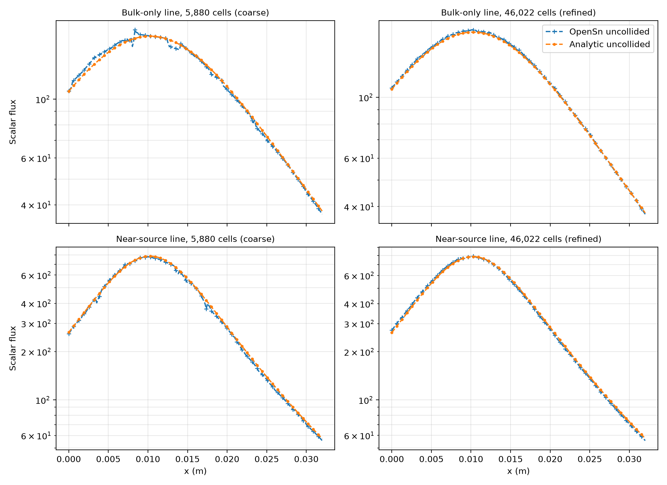
Top row: the bulk-only line from above. Refining from 5,880 to about 46,000 cells reduces its mean relative error from about 2.2% to about 1.0%, and its maximum relative error from about 7.7% to about 2.4% — the jumps visibly shrink and the errors asserted above confirm it numerically rather than only by eye.

Bottom row: a second line, offset only 0.006 m in y and z instead of the 0.0126 m/0.00936 m used above, so it crosses the ray-traced near-source region. Its mean relative error only drops from about 2.7% to about 2.5% under the same refinement — accuracy there is governed by the near-source ray-tracing treatment rather than bulk-cell size, so the improvement is real but far more modest than the bulk-only line’s.