4.2.4. Spatial Convergence
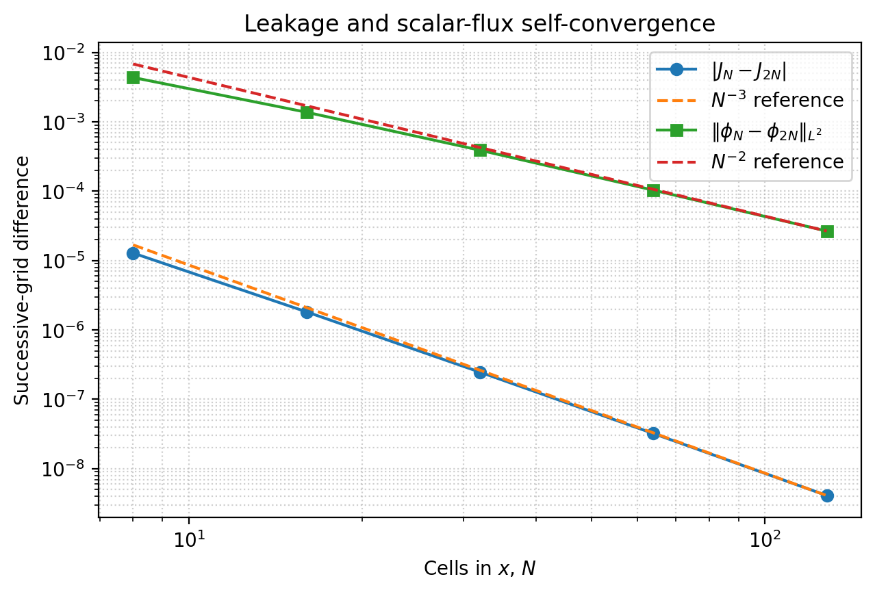
This tutorial separates two spatial-convergence behaviors of OpenSn’s piecewise-linear discontinuous Galerkin (PWLD) discretization: approximately third-order convergence of a right-boundary leakage functional and approximately second-order convergence of the scalar flux in the \(L^2\) norm. The leakage result is a special outflow superconvergence property, not the global order of the flux solution.
4.2.4.1. Define the self-convergence metric
The unit square contains a one-group material with \(\Sigma_t=1\) and scattering ratio \(c=\Sigma_s/\Sigma_t=0.8\). A uniform isotropic source of unit strength is applied throughout the square. The left and right boundaries are vacuum, while the top and bottom boundaries are reflecting. Because the material, source, and boundary conditions are uniform in \(y\), the solution is effectively one-dimensional. We begin with an \(8\times8\) mesh, refine only the \(x\) direction, and hold \(N_y=8\) fixed.
Scattering removes the simple characteristic reference available for a pure absorber. Instead, let \(J_N\) and \(\phi_N\) denote the leakage and scalar flux calculated with \(N\) cells in \(x\). Define the successive-grid differences
The scalar-flux difference is evaluated by elementwise Gaussian quadrature on the finer mesh, so it measures the field itself rather than potentially superconvergent cell averages. If either error behaves as \(Ch^p\), the observed order follows from three successive meshes:
The angular quadrature and iterative-solver tolerance remain fixed so that the measured differences are dominated by spatial refinement toward the fixed-\(S_N\) solution.
[ ]:
import math
import matplotlib.pyplot as plt
from mpi4py import MPI
from pyopensn.aquad import GLCProductQuadrature2DXY
from pyopensn.context import Finalize
from pyopensn.fieldfunc import FieldFunctionInterpolationPoint
from pyopensn.math import Vector3
from pyopensn.mesh import OrthogonalMeshGenerator
from pyopensn.solver import DiscreteOrdinatesProblem, SteadyStateSourceSolver
from pyopensn.source import VolumetricSource
from pyopensn.xs import MultiGroupXS

rank = MPI.COMM_WORLD.rank
quadrature = GLCProductQuadrature2DXY(
    n_polar=2, n_azimuthal=64, scattering_order=0
)

def solve_transport(nx, ny=8):
    x_nodes = [i / nx for i in range(nx + 1)]
    y_nodes = [i / ny for i in range(ny + 1)]
    mesh = OrthogonalMeshGenerator(
        node_sets=[x_nodes, y_nodes]
    ).Execute()
    mesh.SetUniformBlockID(0)

    xs = MultiGroupXS()
    xs.CreateSimpleOneGroup(sigma_t=1.0, c=0.8)
    problem = DiscreteOrdinatesProblem(
        mesh=mesh,
        num_groups=1,
        groupsets=[
            {
                "groups_from_to": (0, 0),
                "angular_quadrature": quadrature,
                "inner_linear_method": "petsc_gmres",
                "l_abs_tol": 1.0e-12,
                "l_max_its": 300,
                "gmres_restart_interval": 100,
            }
        ],
        xs_map=[{"block_ids": [0], "xs": xs}],
        volumetric_sources=[
            VolumetricSource(block_ids=[0], group_strength=[1.0])
        ],
        boundary_conditions=[
            {"name": "xmin", "type": "vacuum"},
            {"name": "xmax", "type": "vacuum"},
            {"name": "ymin", "type": "reflecting"},
            {"name": "ymax", "type": "reflecting"},
        ],
        options={
            "save_angular_flux": True,
            "verbose_inner_iterations": False,
        },
    )
    solver = SteadyStateSourceSolver(problem=problem)
    solver.Initialize()
    solver.Execute()

    leakage = float(problem.ComputeLeakage(["xmax"])["xmax"][0])
    scalar_flux = problem.GetScalarFluxFieldFunction(
        only_scalar_flux=True
    )[0]
    return leakage, scalar_flux


def scalar_flux_l2_difference(coarse_flux, fine_flux, fine_nx, ny=8):
    coarse_interpolator = FieldFunctionInterpolationPoint()
    coarse_interpolator.SetFieldFunction(coarse_flux)
    fine_interpolator = FieldFunctionInterpolationPoint()
    fine_interpolator.SetFieldFunction(fine_flux)

    gauss_points = (-1.0 / math.sqrt(3.0), 1.0 / math.sqrt(3.0))
    dx = 1.0 / fine_nx
    dy = 1.0 / ny
    squared_error = 0.0
    for i in range(fine_nx):
        x_midpoint = (i + 0.5) * dx
        for j in range(ny):
            y_midpoint = (j + 0.5) * dy
            for xi in gauss_points:
                x = x_midpoint + 0.5 * dx * xi
                for eta in gauss_points:
                    y = y_midpoint + 0.5 * dy * eta
                    point = Vector3(x, y, 0.0)
                    coarse_interpolator.SetPointOfInterest(point)
                    coarse_interpolator.Execute()
                    fine_interpolator.SetPointOfInterest(point)
                    fine_interpolator.Execute()
                    difference = (
                        coarse_interpolator.GetPointValue()
                        - fine_interpolator.GetPointValue()
                    )
                    squared_error += (
                        0.25 * dx * dy * difference**2
                    )
    return math.sqrt(squared_error)
4.2.4.2. Refine the mesh
The number of cells in \(x\) is doubled at every level while the eight \(y\) cells are retained. OpenSn’s PWLD formulation uses an upwind angular flux in the surface term. For this smooth, effectively one-dimensional problem, the leakage samples the outgoing trace at its favorable downwind location and approaches third-order superconvergence. Linear DG nevertheless retains its usual approximately second-order convergence for the scalar-flux field in \(L^2\).
The third-order leakage result is specific to this aligned, smooth configuration and response functional. It should not be assumed for arbitrary unstructured meshes, nonsmooth solutions, discontinuous or unaligned material interfaces, or other response functionals. Downwind-point superconvergence of order \(2k+1\) for degree-\(k\) upwind DG methods is discussed by Cao, Zhang, and Zou.
[ ]:
ny = 8
resolutions = [8, 16, 32, 64, 128, 256]
solutions = [
    solve_transport(nx, ny) for nx in resolutions
]
leakage_values = [solution[0] for solution in solutions]
scalar_fluxes = [solution[1] for solution in solutions]

leakage_differences = [
    abs(coarse - fine)
    for coarse, fine in zip(leakage_values, leakage_values[1:])
]
leakage_orders = [
    math.log(
        leakage_differences[index - 1] / leakage_differences[index],
        2.0,
    )
    for index in range(1, len(leakage_differences))
]
scalar_flux_differences = [
    scalar_flux_l2_difference(coarse, fine, fine_nx, ny)
    for coarse, fine, fine_nx in zip(
        scalar_fluxes, scalar_fluxes[1:], resolutions[1:]
    )
]
scalar_flux_orders = [
    math.log(
        scalar_flux_differences[index - 1]
        / scalar_flux_differences[index],
        2.0,
    )
    for index in range(1, len(scalar_flux_differences))
]

if rank == 0:
    for nx, leakage in zip(resolutions, leakage_values):
        print(f"{nx:3d} x {ny:3d} cells: leakage={leakage:.10e}")
    for index, nx in enumerate(resolutions[:-2]):
        print(
            f"{nx:3d}->{2 * nx:3d}->{4 * nx:3d}: "
            f"leakage order={leakage_orders[index]:.6f}, "
            f"scalar-flux L2 order={scalar_flux_orders[index]:.6f}"
        )
    print(
        "Spatial-convergence leakage final order="
        f"{leakage_orders[-1]:.6e}"
    )
    print(
        "Spatial-convergence leakage final difference="
        f"{leakage_differences[-1]:.6e}"
    )
    print(
        "Spatial-convergence scalar-flux final order="
        f"{scalar_flux_orders[-1]:.6e}"
    )
    print(
        "Spatial-convergence scalar-flux final difference="
        f"{scalar_flux_differences[-1]:.6e}"
    )
assert all(
    fine < coarse
    for coarse, fine in zip(
        leakage_differences, leakage_differences[1:]
    )
)
assert all(
    fine < coarse
    for coarse, fine in zip(
        scalar_flux_differences, scalar_flux_differences[1:]
    )
)
assert min(leakage_orders) > 2.8
assert 1.9 < scalar_flux_orders[-1] < 2.1
4.2.4.3. Interpret and plot the convergence
The observed leakage orders approach three, while the scalar-flux \(L^2\) orders approach two. This confirms that the unusually high leakage order belongs to the outgoing response functional and does not describe the accuracy of the full spatial solution.
The successive-grid leakage and scalar-flux \(L^2\) differences are plotted against the coarser \(x\) resolution. The dashed \(N^{-3}\) and \(N^{-2}\) lines illustrate their distinct asymptotic behaviors. The committed figure below was generated by this cell; uncomment fig.savefig(...) to regenerate it after changing the problem.
[ ]:
if rank == 0:
    comparison_resolutions = resolutions[:-1]
    third_order = [
        leakage_differences[-1]
        * (comparison_resolutions[-1] / nx) ** 3
        for nx in comparison_resolutions
    ]
    second_order = [
        scalar_flux_differences[-1]
        * (comparison_resolutions[-1] / nx) ** 2
        for nx in comparison_resolutions
    ]

    fig, ax = plt.subplots(figsize=(6.5, 4.5))
    ax.loglog(
        comparison_resolutions,
        leakage_differences,
        "o-",
        label=r"$|J_N-J_{2N}|$",
    )
    ax.loglog(
        comparison_resolutions,
        third_order,
        "--",
        label=r"$N^{-3}$ reference",
    )
    ax.loglog(
        comparison_resolutions,
        scalar_flux_differences,
        "s-",
        label=r"$\|\phi_N-\phi_{2N}\|_{L^2}$",
    )
    ax.loglog(
        comparison_resolutions,
        second_order,
        "--",
        label=r"$N^{-2}$ reference",
    )
    ax.set_xlabel("Cells in $x$, $N$")
    ax.set_ylabel("Successive-grid difference")
    ax.set_title("Leakage and scalar-flux self-convergence")
    ax.grid(True, which="both", linestyle=":", alpha=0.6)
    ax.legend()
    fig.tight_layout()
    # fig.savefig("images/spatial_convergence.png", dpi=200, bbox_inches="tight")

if "opensn_console" not in globals():
    from IPython import get_ipython
    if get_ipython() is not None:
        Finalize()
        MPI.Finalize()