2. Phase-space Discretization

2.1. Energy Discretization

The energy interval \(\mathcal{E}=[0,E_{\text{max}}]\) is subdivided into energy groups \([E_g,E_{g-1}]\) (\(1 \le g \le G\)), where \(G\) is the total number of groups and with the convention that \(E_g < E_{g-1}\) so faster energy groups have smaller indices.

Integration in energy of the energy-continuous linear Boltzmann equation over each group \(g\) yields \(G\) equations that are coupled through the angle-energy distribution/scattering term:

\[\begin{split}\begin{gathered} \frac{1}{v^g} \frac{\partial \psi^g(\vec{r},\vec{\Omega},t)}{\partial t} + \vec{\Omega} \cdot \vec{\nabla} \psi^g(\vec{r},\vec{\Omega},t) + \sigma_t^g(\vec{r},t)\psi^g(\vec{r},\vec{\Omega},t) \\= \sum_{g'=1}^{g'=G} \sum_{\ell=0}^{L_{\text{max}}} \sum_{m=-\ell}^{m=\ell} \, \frac{2\ell+1}{4\pi}\sigma^{g'\to g}_{s,\ell}(\vec{r},t) Y_{\ell,m}(\vec{\Omega}) \phi^{g'}_{\ell,m}(\vec{r},t) + Q^g_{\text{ext}}(\vec{r},\vec{\Omega},t) \end{gathered}\end{split}\]

for all \(1\le g \le G\). The multigroup energy discretization can be thought of as a finite-volume discretization in energy. When fission is present, the above equation is amended to account for the additional fission production term.

The multigroup fluxes are the energy-dependent fluxes integrated over the energy group. For example,

\[\psi^g(\vec{r},\vec{\Omega},t) = \int_{E_g}^{E_{g-1}} dE \,\psi(\vec{r},\vec{\Omega},E,t) \,,\]

and likewise for flux moments

\[\phi^{g}_{\ell,m}(\vec{r},t) = \int_{E_g}^{E_{g-1}} dE \, \phi_{\ell,m}(\vec{r},E,t) \,.\]

Adequately energy-averaged multigroup cross sections must be supplied to OpenSn. See the Theory section on multigroup cross sections for additional details.

In the remainder of this theory manual, we focus on the steady-state linear Boltzmann equation, for brevity:

\[\begin{split}\begin{gathered} \vec{\Omega} \cdot \vec{\nabla} \psi^g(\vec{r},\vec{\Omega}) + \sigma_t^g(\vec{r})\psi^g(\vec{r},\vec{\Omega}) \\= \sum_{g'=1}^{g'=G} %\sum_{\ell=0}^{L_{\text{max}}} \sum_{m=-\ell}^{m=\ell} \sum_{\ell,m} \, \frac{2\ell+1}{4\pi}\sigma^{g'\to g}_{s,\ell}(\vec{r}) Y_{\ell,m}(\vec{\Omega}) \phi^{g'}_{\ell,m}(\vec{r}) + Q^g_{\text{ext}}(\vec{r},\vec{\Omega}) \\ \qquad 1\le g \le G \,. \end{gathered}\end{split}\]

The summation on indices \(\ell\) and \(m\) is to be understood as a double summation. The summation on \(\ell\) goes from 0 to \(L_\text{max}\). The summation in \(m\) depends on the dimensionality of the problem. In 1D, there is no summation on \(m\) (equivalent to setting \(m=0\)), in 2D, the summation on \(m\) is from 0 to \(\ell\) and in 3D, the summation on \(m\) is from \(-\ell\) to \(\ell\).

We will further consider a single one of the above \(G\) equations, written without the group superscript \(g\) for conciseness:

\[\vec{\Omega} \cdot \vec{\nabla} \psi(\vec{r},\vec{\Omega}) + \sigma_t(\vec{r})\psi(\vec{r},\vec{\Omega})= %\sum_{\ell=0}^{L_{\text{max}}} \sum_{m=-\ell}^{m=\ell} \sum_{\ell,m} \, \frac{2\ell+1}{4\pi}\sigma_{s,\ell}(\vec{r}) Y_{\ell,m}(\vec{\Omega}) \phi_{\ell,m}(\vec{r}) + Q(\vec{r},\vec{\Omega}) \,,\]

where the source term \(Q(\vec{r},\vec{\Omega})\) is now the sum of the external source and the upscattering and downscattering contributions to the current group \(g\).

2.2. Angle Discretization (the Sn method)

The \(S_n\) discrete-ordinate method Carlson and Bell [CB58], Carlson and Lee [CL61], Lee [Lee61], Lathrop and Carlson [LC64], Carlson and Lathrop [CL65], Carlson [Car71], Gelbard et al. [GDH69] is a collocation in angle approach, where a set of fixed (discrete) directions \(\vec{\Omega}_d\) are chosen. In order to evaluate angular integrals to compute the flux moments \(\phi_{\ell,m}\), weights \(\omega_d\) associated with each discrete direction are also defined. It is therefore customary to discuss the \(S_n\) method using the notion of angular quadratures.

Given an angular quadrature rule with \(N_{\text{dir}}\) directions and weights

\[\left( \vec{\Omega}_d, \omega_d \right) \qquad \text{with } 1 \le d \le N_{\text{dir}}\]

the one-group transport equation (REF above) devolves into a set of \(N_{\text{dir}}\) coupled equations, with the coupling occurring through the scattering (redistribution in angle) term:

\[\begin{split}\begin{gathered} \vec{\Omega}_d \cdot \vec{\nabla} \psi_d(\vec{r}) + \sigma_t(\vec{r})\psi_d(\vec{r})= \sum_{\ell,m}\, \frac{2\ell+1}{4\pi}\sigma_{s,\ell}(\vec{r}) Y_{\ell,m}(\vec{\Omega}_d) \phi_{\ell,m}(\vec{r}) + Q_d(\vec{r}) \\ \qquad \text{for } 1 \le d \le N_{\text{dir}}\,, \end{gathered}\end{split}\]

with \(\psi_d(\vec{r}) \equiv \psi(\vec{r},\vec{\Omega}_d)\) and \(Q_d(\vec{r}) \equiv Q(\vec{r},\vec{\Omega}_d)\).

In order to evaluate flux moments, we use the quadrature rule:

\[\phi_{\ell,m}(\vec{r}) \simeq \sum_{d=1}^{N_{\text{dir}}} \omega_d Y_{\ell,m}(\vec{\Omega}_d) \psi_d(\vec{r}) \,.\]

We can now define the entries in the \(M\) and \(D\) matrices introduced earlier:

• the discrete-to-moment matrix:

  \[M_{k,d} = \omega_d Y_{\ell,m}(\vec{\Omega}_d)\]

  where \(k\) is a single index encoding the pair \((\ell,m)\). The dimensions of \(M\) are: \(N_{\text{mom}} \times N_{\text{dir}}\).

• the moment-to-discrete matrix:

  \[D_{d,k} = \frac{2\ell+1}{4\pi} Y_{\ell,m}(\vec{\Omega}_d)\]

  The dimensions of \(D\) are: \(N_{\text{dir}} \times N_{\text{mom}}\).

Traditional quadrature rules include the Level-Symmetric quadrature, the Equal-Weight quadrature, and Gauss-Legendre-Chebyshev quadratures. In OpenSn, we have:

1. the Product Gauss-Legendre-Chebyshev quadrature, which is the tensor product of a Gauss-Legendre quadrature in polar angle \(\mu\) and a Gauss-Chebyshev quadrature in azimuthal angle \(\varphi\). When the number of discrete positive polar angles is equal to the number of discrete azimuthal angles in one quadrant, the Product Gauss-Legendre-Chebyshev quadrature is said to the square; otherwise it is said to be rectangular. The number of directions in one octant of the unit sphere is

   \[N_{\text{polar}} \times N_{\text{azimuthal}}\]

   where \(N_{\text{polar}}\) is the number of positive polar angles and \(N_{\text{azimuthal}}\) is the number of azimuthal angles in one quadrant.

   

   Product Gauss-Legendre-Chebyshev quadrature (\(N_{\text{polar}}=N_{\text{azimuthal}}=4\))

   

   Product Gauss-Legendre-Chebyshev quadrature (\(N_{\text{polar}}=N_{\text{azimuthal}}=6\))

2. the Triangle Gauss-Legendre-Chebyshev quadrature is similar to the Product Gauss-Legendre-Chebyshev quadrature. However, the number of azimuthal angles per quadrant depends on the polar level: at the most equatorial polar level, the number of azimuthal angles per quadrant is \(N_{\text{polar}}\); at each successive polar level, the number of azimuthal angles per quadrant is one less to finally reach one azimuthal angle per quadrant at the polar level closest to the pole. The number of directions in one octant of the unit sphere is

   \[\frac{N_{\text{polar}} (N_{\text{polar}}+1)}{2}\]

   

   Triangular Gauss-Legendre-Chebyshev quadrature (\(N_{\text{polar}}=4\))

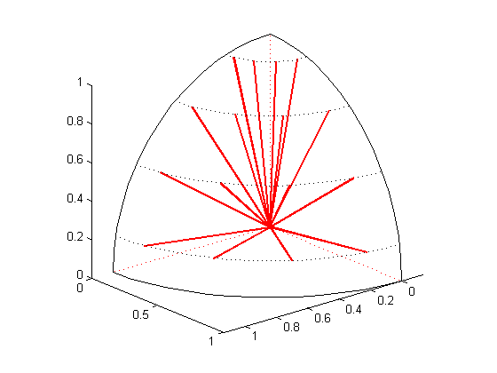
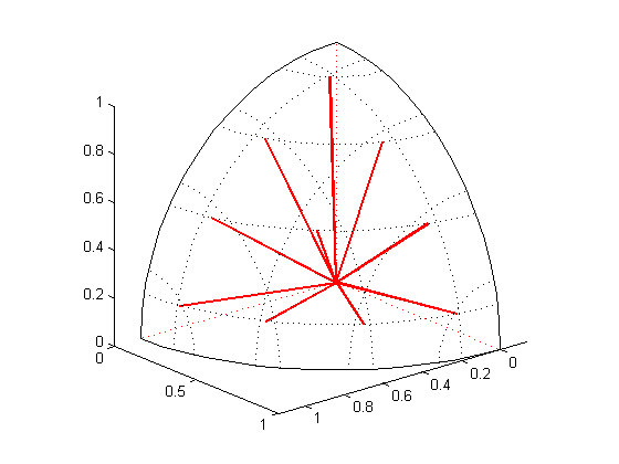
3. the LDFE (linear discontinuous finite-element in angle Lau and Adams [LA17]) quadrature, using spherical quadrilaterals. The LDFE quadrature divides one octant of the unit sphere into spherical quadrilaterals. The quadrature directions are then the 4 Gauss-Legendre points per quadrilateral and the weights are computed to obtain 4-th order accuracy. Note that the quadrilateral can be easily subdivided into 4 smaller quadrilaterals, hence yielding a locally refined angular quadrature.

   

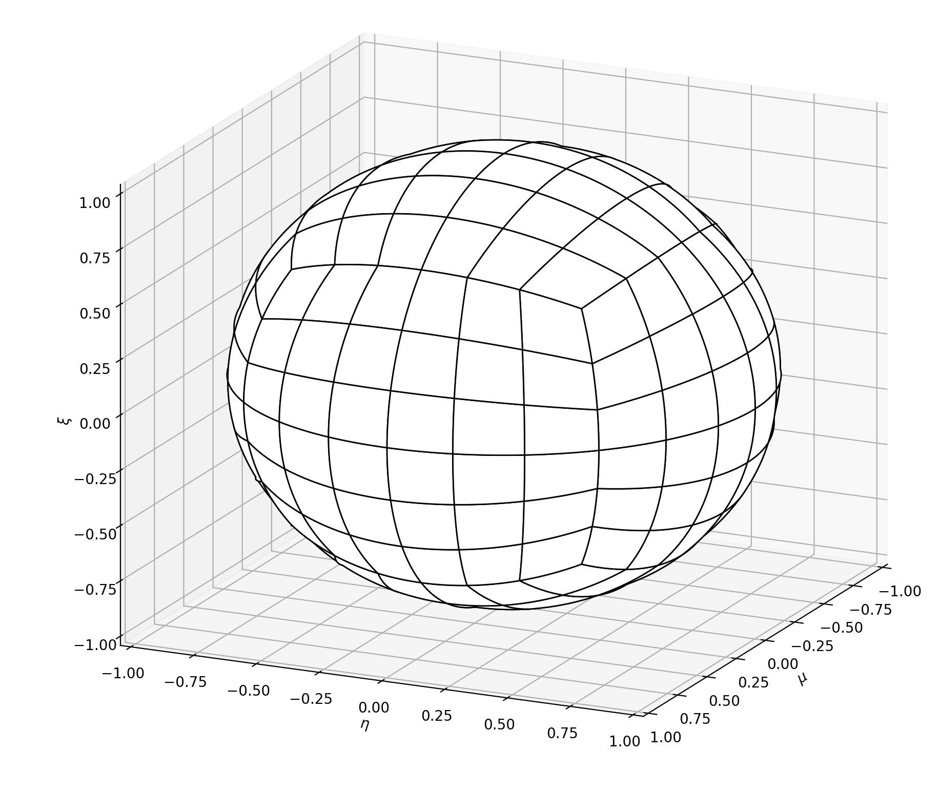
   Example of uniform LDFE angular quadrature

   

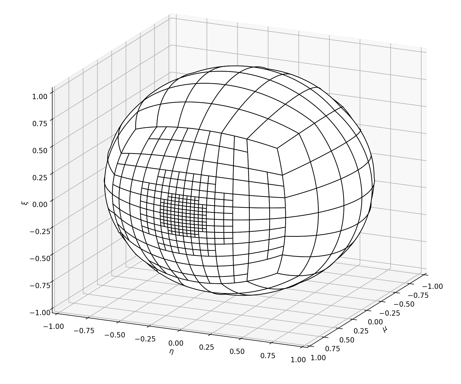
   Example of locally refined LDFE angular quadrature

4. The user has has the option of supplying their own quadrature rule.

For charged-particle transport, not yet covered in OpenSn, Galerkin variants of the traditional quadrature rules must be employed Morel [Mor89], Sanchez and Ragusa [SR11].

Note that any discrete-ordinate \(S_n\) method can produce “ray effects” due to angular discretization errors Lathrop [Lat68], Lathrop [Lat71], Morel et al. [MWLP03], Miller Jr and Reed [MJR77]. These errors are most pronounced in situations with low scattering materials, low density materials, and in presence of small localized sources, … An uncollided-flux approach is often employed to mitigate ray effects. See the section on the uncollided-flux approach for additional details .

2.3. Spatial Discretization

In this section, we describe the Discontinuous Galerkin Finite Element Method (DGFEM) applied to the linear Boltzmann equation on meshes made of arbitrary polyhedra in 3D and arbitrary polygons in 2D. For references on DGFEM applied to transport, please consult Reed and Hill [RH73], Lesaint and Raviart [LR74], Hill [Hil75], Reed et al. [RHBL73], Seed et al. [SMJBJ77], Seed et al. [SMB78], Adams [Ada01], Wareing et al. [WMMP01], Morel and Warsa [MW05], Wang and Ragusa [WR09a], Wang and Ragusa [WR09b], Wang [Wan09], Wang and Ragusa [WR11], Wang and Ragusa [WR10].

For a given energy group (\(g\) index omitted for brevity) and for a given angular direction \(d\), the transport equation is

\[\vec{\Omega}_d \cdot \vec{\nabla} \psi_d(\vec{r}) + \sigma_t(\vec{r})\psi_d(\vec{r})= \sum_{\ell,m} \, \frac{2\ell+1}{4\pi}\sigma_{s,\ell}(\vec{r}) Y_{\ell,m}(\vec{\Omega}_d) \phi_{\ell,m}(\vec{r}) + Q_d(\vec{r}) \equiv q_d(\vec{r}) \,,\]

where the total source term \(q_d\) includes all source terms (within-group scattering, external, and inscattering from other groups).

A mesh \(T_{h}\) is used to discretize the domain \(\mathcal{D}\) into arbitrary elements \(K\), such that the union of the all elements fully covers \(\mathcal{D}\), i.e., \(\bigcup\nolimits_{K\in T_{h}} K =\mathcal{D}.\) We assume that the boundary of \(\mathcal{D}\) consists of planar faces.

For the purpose of writing the bilinear form of the DGFEM formulation, we now introduce the volume and surface inner products on any element \(K\) and its boundary \(\partial K\), respectively,

\[\begin{split}\begin{aligned} (f,g)_{K} &=& \int_{K} d^{3}r \, f(\vec{r}) g(\vec{r}), \\ (f,g)_{\partial K} &=& \int_{\partial K} d^{2}r \, | \vec{\Omega} \cdot \vec{n}(\vec{r}) | f(\vec{r}) g(\vec{r}). \end{aligned}\end{split}\]

In the case of 3D geometries, these products are to be understood as volume and surface integrals.

The DGFEM applied to the transport equation is obtained by multiplying it by a (discontinuous) test function \(b_{i}\) and integrating the result over each element, i.e.,

\[\begin{split}\begin{aligned} &&\sum\limits_{K\in T_{h}}\left\{ -(\vec{\Omega }_d\cdot \vec{\nabla }b_{i}\,,\,\psi_d )_{K} + (b_{i}\,,\,\sigma_t \psi_d )_{K}+(\psi_d^{+} \, , \,b_{i}^{+})_{\partial K^{+}} \right\} \notag \\ &&\qquad=\ \sum\limits_{K\in T_{h}}\left\{ (q_d\,,\,b_{i})_{K} +(\psi_d ^{-}\, ,\,b_{i}^{+})_{\partial K^{-}}\right\} \,, \label{eq:DGFEM-v1} \end{aligned}\end{split}\]

where \(\partial K^{-}\) is the inflow boundary for cell \(K\) (\(\partial K^{-}=\{x\in \partial K\) such that \(\vec{\Omega }\cdot \vec{n}<0\}\)), \(\partial K^{+}\) is the outflow boundary for cell \(K\) (\(\partial K^{+}=\{x\in \partial K\) such that \(\vec{\Omega }\cdot \vec{n}>0\}\)), \(f^{+}\) denotes the restriction of any function \(f\) taken from within element \(K\) and \(f^{-}\) represents the restriction of \(f\) taken from the neighboring element of \(K\).

The left-hand-side integrals contain the angular flux unknowns for each element \(K\), whereas the right-hand-side integrals contain the radiation contribution to cell \(K\), from both (i) the volumetric source contribution \(q\) but also (ii) the inflow radiation from the incoming cell boundaries. The latter term uses the upwind flux \(\psi_d ^{-}\), i.e., the angular flux from the neighboring upwind elements. When an element lies on the domain boundary \(\Gamma\), the incoming contribution is supplied by boundary conditions.

Transport sweeps and task-directed graphs It is important to note that, with a DGFEM discretization, the small linear system associated with cell \(K\) can be solved for the angular flux \(\psi_d\) in cell \(K\) as soon as the upwind contributions are known. This means that, given a proper ordering of the elements \(K\) in a task-directed graph (TDG) for direction \(\vec{\Omega}_d\), the global system can be solved cell-by-cell, by traversing the TDG.

Example of a transport sweep sequence

It is possible that the TDG presents some cycles on unstructured grids. In this case, cycles are broken based on the smallest values of \(| \vec{\Omega} \cdot \vec{n}(\vec{r}) |\) for the incoming faces causing the cycle. The angular flux contributions to those faces are lagged and iterated upon until convergence.

Piece-Wise Linear (PWL) basis functions on arbitrary polyhedra Stone and Adams [SA03], Bailey [Bai08], Bailey et al. [BACW08], Warsa [War08], Ragusa [Rag15]: PWL basis functions are defined such that they are equal to one on a single vertex and zero on all other vertices. Their construction is achieved by splitting each polyhedron into several tetrahedra. However, note that the number of unknowns associated with a given polyhedron is always equal to its number of vertices, and not to the number of vertices in the underlying tetrahedra. The tetrahedra are constructed by taking two neighboring vertices of the polyhedron, the face centroid of a face of the polyhedron containing the two chosen vertices, and the polyhedron centroid.

On each tetrahedron, standard linear finite element basis functions are defined, as \(t_j(\vec{r})\) where \(j\) is any vertex of the polyhedron: \(t_j(\vec{r})\) equals 1 at the \(j\)-th vertex of the polyhedron and decreases linearly to zero on all other vertices connected to vertex \(j\) by an edge. We also define an interior function \(t_c(\vec{r})\) that is unity at the polyhedron centroid and zero at each face midpoint and polyhedron cell vertex. The polyhedron centroid is defined as

\[\vec{r}_c = \frac{1}{N_v} \sum_{j=1}^{N_v} \vec{r}_j\]

with \(N_v\) the number of cell vertices of the polyhedron. Finally we define face functions \(t_f(\vec{r})\) that are unity at the face centroid and zero at the polyhedron’s centroid and at each of the face’s vertices. A face centroid is defined as

\[\vec{r}_f = \frac{1}{N_f} \sum_{j=1}^{N_f} \vec{r}_j\]

with \(N_f\) the number of face vertices for face \(f\) of the polyhedron.

Then, the PWL basis function associated with vertex \(j\) is:

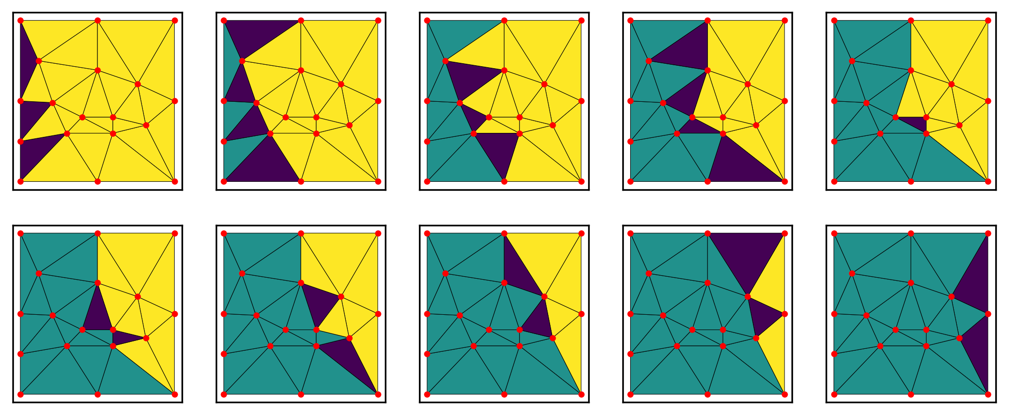
\[b_j(\vec{r}) = t_j(\vec{r}) + \frac{1}{N_f}\sum_{f @ j} t_f(\vec{r}) + \frac{1}{N_v}t_c(\vec{r})\]

where \(f @ j\) denotes a face containing vertex \(j\). It is easy to check that \(b_j(\vec{r})\) is equal to one on vertex \(j\) of the polyhedron and zero on all its other vertices.

PWL basis functions in 2D for an arbitrary pentagon

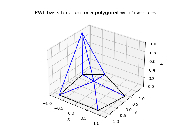
A PWL basis function in 2D for a degenerated square (pentagon).

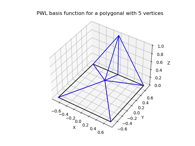
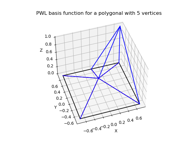
Another PWL basis function in 2D for a degenerated square (pentagon).

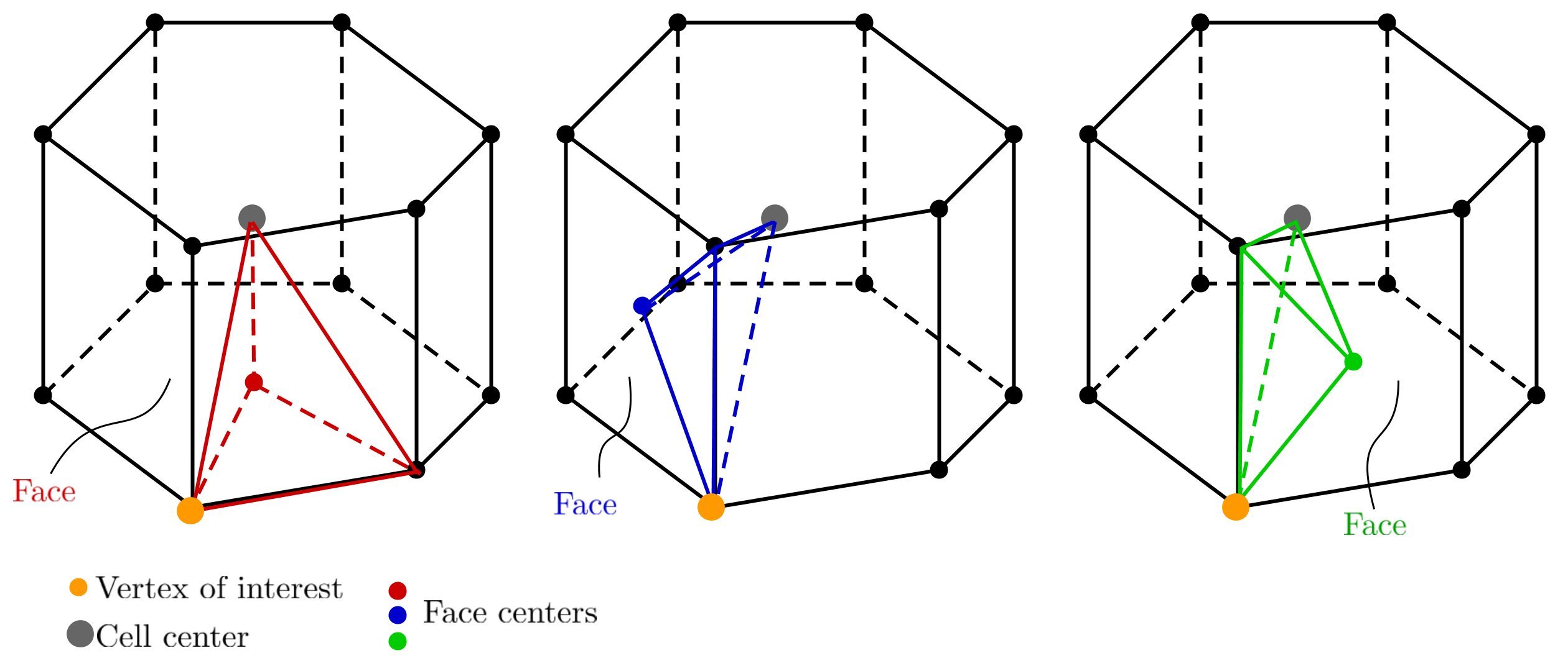
Identification of PWL basis functions in 3D

The various local matrices appearing in the local DGFEM systems are built using the PWL basis functions. Their integrals are computed using a spatial numerical quadrature per tetrahedron mapped on to the reference tetrahedron. These matrices are computed only once and then stored. The volumetric and surface leakage matrices are computed and stored before applying the angular direction \(\vec{\Omega}\) and the mass matrices are computed and stored before applying the cross-section values. Hence, the number of matrices stored only depends on the mesh (total number of polyhedral cells, total number of faces) and not on the number of energy groups used nor the number of directions employed.

2.4. References

[CB58]

BG Carlson and GI Bell. Solution of the transport equation by the sn method. Technical Report, Los Alamos Scientific Lab., N. Mex., 1958.

[CL61]

Bengt G Carlson and Clarence E Lee. Mechanical quadrature and the transport equation. Volume 2573. Los Alamos Scientific Laboratory of the University of California, 1961.

[Lee61]

Clarence E Lee. The discrete $s_n$ approximation to transport theory. Technical Report, Los Alamos Scientific Lab., N. Mex., 1961.

[LC64]

Kaye D Lathrop and Bengt G Carlson. Discrete ordinates angular quadrature of the neutron transport equation. Technical Report, Los Alamos Scientific Lab., N. Mex., 1964.

[CL65]

Bengt G Carlson and Kaye D Lathrop. Transport theory: the method of discrete ordinates. Los Alamos Scientific Laboratory of the University of California, 1965.

[Car71]

BG Carlson. On a more precise definition of discrete ordinates methods. In Proceedings of the Second Conference on Transport Theory, 348–390. U.S. Atomic Energy Commission, 1971.

[GDH69]

EM Gelbard, James A Davis, and LA Hageman. Solution of the discrete ordinate equations in one and two dimensions. Transport Theory, 1:129–158, 1969.

[LA17]

Cheuk Y. Lau and Marvin L. Adams. Discrete ordinates quadratures based on linear and quadratic discontinuous finite elements over spherical quadrilaterals. Nuclear Science and Engineering, 185(1):36–52, 2017. URL: https://doi.org/10.13182/NSE16-28, doi:10.13182/NSE16-28.

[Mor89]

Jim E Morel. A hybrid collocation-galerkin-sn method for solving the boltzmann transport equation. Nuclear Science and Engineering, 101(1):72–87, 1989.

[SR11]

Richard Sanchez and Jean Ragusa. On the construction of galerkin angular quadratures. Nuclear Science and Engineering, 169(2):133–154, 2011. URL: https://doi.org/10.13182/NSE10-31, doi:10.13182/NSE10-31.

[Lat68]

K D Lathrop. Ray effects in discrete ordinates equations. Nuclear Science and Engineering, 32(3):357–369, 1968.

[Lat71]

KD Lathrop. Remedies for ray effects. Nuclear Science and Engineering, 45(3):255–268, 1971.

[MWLP03]

J.E. Morel, T.A. Wareing, R.B. Lowrie, and D.K. Parsons. Analysis of ray-effect mitigation techniques. Nuclear Science and Engineering, 144:1–22, 2003.

[MJR77]

WF Miller Jr and Wm H Reed. Ray-effect mitigation methods for two-dimensional neutron transport theory. Nuclear Science and Engineering, 62(3):391–411, 1977.

[RH73]

Wm H Reed and TR Hill. Triangular mesh methods for the neutron transport equation. Los Alamos Report LA-UR-73-479, 1973.

[LR74]

P Lesaint and PA Raviart. On a finite element method for solving the neutron transport equation. Mathematical Aspects of Finite Elements in Partial Differential Equations, pages 89–123, 1974.

[Hil75]

TR Hill. Onetran: a discrete ordinates finite element code for the solution of the one-dimensional multigroup transport equation (la-5990-ms). Technical Report, Los Alamos Scientific Lab., N. Mex.(USA), 1975.

[RHBL73]

Wm H Reed, TR Hill, FW Brinkley, and KD Lathrop. Triplet: a two-dimensional, multigroup, triangular mesh, planar geometry, explicit transport code. Technical Report, Los Alamos Scientific Lab., N. Mex.(USA), 1973.

[SMJBJ77]

TJ Seed, WF Miller Jr, and FW Brinkley Jr. Trident: a two-dimensional, multigroup, triangular mesh discrete ordinates, explicit neutron transport code. Technical Report, Los Alamos Scientific Lab., NM (USA), 1977.

[SMB78]

TJ Seed, WF Miller, and GE Bosler. Trident: a new triangular mesh discrete ordinates code. In ANS Meeting, 157–167. 1978.

[Ada01]

Marvin L Adams. Discontinuous finite element transport solutions in thick diffusive problems. Nuclear Science and Engineering, 137(3):298–333, 2001.

[WMMP01]

Todd A Wareing, John M McGhee, Jim E Morel, and Shawn D Pautz. Discontinuous finite element $s_n$ methods on three-dimensional unstructured grids. Nuclear Science and Engineering, 138(3):256–268, 2001.

[MW05]

Jim E Morel and James S Warsa. An $s_n$ spatial discretization scheme for tetrahedral meshes. Nuclear Science and Engineering, 151(2):157–166, 2005.

[WR09a]

Yaqi Wang and Jean C Ragusa. On the convergence of dgfem applied to the discrete ordinates transport equation for structured and unstructured triangular meshes. Nuclear Science and Engineering, 163(1):56–72, 2009.

[WR09b]

Yaqi Wang and Jean C Ragusa. A high-order discontinuous galerkin method for the $s_n$ transport equations on 2d unstructured triangular meshes. Annals of Nuclear Energy, 36(7):931–939, 2009.

[Wan09]

Yaqi Wang. Adaptive mesh refinement solution techniques for the multigroup $S_N$ transport equation using a higher-order discontinuous finite element method. PhD thesis, Texas A&M University, 2009.

[WR11]

Yaqi Wang and Jean C Ragusa. Standard and goal-oriented adaptive mesh refinement applied to radiation transport on 2d unstructured triangular meshes. Journal of Computational Physics, 230(3):763–788, 2011.

[WR10]

Yaqi Wang and Jean C Ragusa. A two-mesh adaptive mesh refinement technique for $s_n$ neutral-particle transport using a higher-order dgfem. Journal of Computational and Applied Mathematics, 233(12):3178–3188, 2010.

[SA03]

Hiromi G Stone and Marvin L Adams. A piecewise linear finite element basis with application to particle transport. In Proc. ANS Topical Meeting Nuclear Mathematical and Computational Sciences Meeting. 2003.

[Bai08]

Teresa S Bailey. The piecewise linear discontinuous finite element method applied to the RZ and XYZ transport equations. PhD thesis, Texas A&M University, 2008.

[BACW08]

Teresa S Bailey, Marvin L Adams, Jae H Chang, and James S Warsa. A piecewise linear discontinuous finite element spatial discretization of the transport equation in 2d cylindrical geometry. In Proc. International Conference on Mathematics and Computational Methods & Reactor Physics, 3–7. 2008.

[War08]

James Warsa. A continuous finite element-base, discontinuous finite element method for $s_n$ transport. Nuclear Science and Engineering, 160:385–400, 2008.

[Rag15]

Jean C. Ragusa. Discontinuous finite element solution of the radiation diffusion equation on arbitrary polygonal meshes and locally adapted quadrilateral grids. Journal of Computational Physics, 280:195–213, 2015. URL: https://www.sciencedirect.com/science/article/pii/S0021999114006494, doi:https://doi.org/10.1016/j.jcp.2014.09.013.