3.1.4. A Two-Dimensional Checkerboard Problem
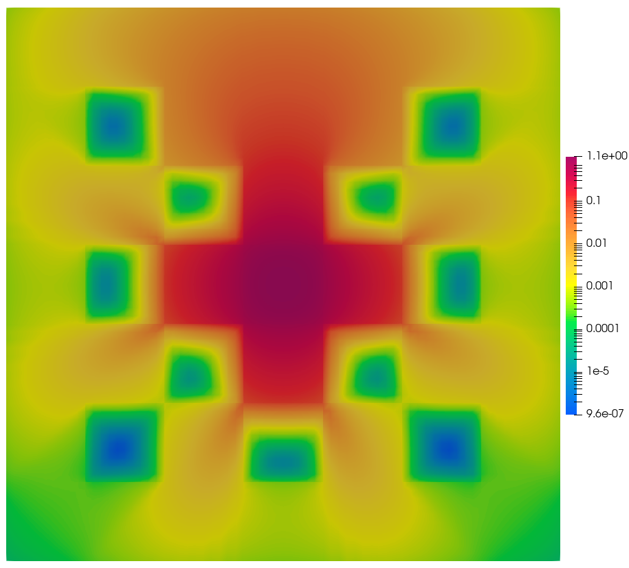
This example places a unit isotropic source at the center of a purely scattering square and surrounds it with a checkerboard pattern of strong absorbers. Particles can scatter through the background, be removed in one of the absorbing squares, or leak through the vacuum exterior boundaries.
3.1.4.1. Import the OpenSn objects
[ ]:
if "opensn_console" not in globals():
    from mpi4py import MPI
    from pyopensn.aquad import GLCProductQuadrature2DXY
    from pyopensn.context import Finalize, UseColor
    from pyopensn.logvol import RPPLogicalVolume
    from pyopensn.mesh import OrthogonalMeshGenerator
    from pyopensn.post import VolumePostprocessor
    from pyopensn.solver import DiscreteOrdinatesProblem, SteadyStateSourceSolver
    from pyopensn.source import VolumetricSource
    from pyopensn.xs import MultiGroupXS

    rank = MPI.COMM_WORLD.rank
    UseColor(False)
3.1.4.2. Create the mesh
The domain is a \(7 \times 7\) cm square discretized with ten cells per centimeter, ensuring that mesh nodes align with every edge of the one-centimeter material squares.
[ ]:
domain_length = 7.0
cells_per_cm = 10
num_cells = int(domain_length * cells_per_cm)
nodes = [i / cells_per_cm for i in range(num_cells + 1)]

mesh = OrthogonalMeshGenerator(node_sets=[nodes, nodes]).Execute()
mesh.SetOrthogonalBoundaries()

BACKGROUND = 0
ABSORBER = 1
SOURCE = 2
mesh.SetUniformBlockID(BACKGROUND)
3.1.4.3. Assign the checkerboard regions
Eleven squares are pure absorbers with \(\sigma_t=\sigma_a=10\) \(\text{cm}^{-1}\).
The background and source square (black) are pure scatterers with \(\sigma_t=\sigma_s=1\) \(\text{cm}^{-1}\).
The source square occupies \([3,4]\times[3,4]\) cm and carries a unit source.
Each tuple below is the lower-left corner of a one-centimeter absorber square. Assigning the source its own block ID allows source selection and postprocessing without changing its material properties.

[ ]:
absorber_origins = [
    (1.0, 1.0), (3.0, 1.0), (5.0, 1.0),
    (2.0, 2.0), (4.0, 2.0),
    (1.0, 3.0), (5.0, 3.0),
    (2.0, 4.0), (4.0, 4.0),
    (1.0, 5.0), (5.0, 5.0),
]

for x_min, y_min in absorber_origins:
    absorber_square = RPPLogicalVolume(
        xmin=x_min, xmax=x_min + 1.0,
        ymin=y_min, ymax=y_min + 1.0,
        infz=True,
    )
    mesh.SetBlockIDFromLogicalVolume(
        absorber_square, ABSORBER, True
    )

source_region = RPPLogicalVolume(
    xmin=3.0, xmax=4.0,
    ymin=3.0, ymax=4.0,
    infz=True,
)
mesh.SetBlockIDFromLogicalVolume(source_region, SOURCE, True)
3.1.4.4. Define the materials and source
The source and background block IDs map to the same scattering cross section. The source is therefore distinguished only by VolumetricSource, not by its transport properties.
[ ]:
scattering_xs = MultiGroupXS()
scattering_xs.CreateSimpleOneGroup(sigma_t=1.0, c=1.0)

absorber_xs = MultiGroupXS()
absorber_xs.CreateSimpleOneGroup(sigma_t=10.0, c=0.0)

source = VolumetricSource(
    block_ids=[SOURCE], group_strength=[1.0]
)
3.1.4.5. Assemble and solve the transport problem
The angular quadrature matches the resolution used by the two-dimensional Reed example. Vacuum conditions on all four exterior faces allow particles that avoid the absorbers to leave the domain.
[ ]:
quadrature = GLCProductQuadrature2DXY(
    n_polar=2, n_azimuthal=64, scattering_order=0
)

problem = DiscreteOrdinatesProblem(
    mesh=mesh,
    num_groups=1,
    groupsets=[
        {
            "groups_from_to": (0, 0),
            "angular_quadrature": quadrature,
            "inner_linear_method": "petsc_gmres",
            "l_abs_tol": 1.0e-9,
            "l_max_its": 300,
            "gmres_restart_interval": 30,
        }
    ],
    xs_map=[
        {"block_ids": [BACKGROUND, SOURCE], "xs": scattering_xs},
        {"block_ids": [ABSORBER], "xs": absorber_xs},
    ],
    volumetric_sources=[source],
    boundary_conditions=[
        {"name": "xmin", "type": "vacuum"},
        {"name": "xmax", "type": "vacuum"},
        {"name": "ymin", "type": "vacuum"},
        {"name": "ymax", "type": "vacuum"},
    ],
)

solver = SteadyStateSourceSolver(problem=problem, compute_balance=True)
solver.Initialize()
solver.Execute()
3.1.4.6. Integrate the source-region flux and absorber reaction rate
The first postprocessor computes the total scalar flux in the black source square,
The second restricts the integral to the absorbing squares block ID and multiplies the flux by the local absorption cross section,
Since the background and source regions are pure scatterers, this block-restricted reaction rate must equal the global absorption rate.
[ ]:
source_flux_postprocessor = VolumePostprocessor(
    problem=problem, value_type="integral", block_ids=[SOURCE]
)
source_flux_postprocessor.Execute()
source_region_flux = source_flux_postprocessor.GetValue()[0][0]

absorption_postprocessor = VolumePostprocessor(
    problem=problem,
    value_type="integral",
    block_ids=[ABSORBER],
    xs_multiplier="sigma_a",
)
absorption_postprocessor.Execute()
black_absorption_rate = absorption_postprocessor.GetValue()[0][0]

balance = solver.ComputeBalanceTable()
source_rate = balance["production_rate"] + balance["inflow_rate"]
loss_rate = balance["absorption_rate"] + balance["outflow_rate"]
relative_balance_error = abs(source_rate - loss_rate) / source_rate

if rank == 0:
    print(f"CHECKERBOARD_SOURCE_REGION_FLUX={source_region_flux:.8e}")
    print(f"CHECKERBOARD_BLACK_ABSORPTION_RATE={black_absorption_rate:.8e}")
    print(f"CHECKERBOARD_BALANCE_ERROR={relative_balance_error:.8e}")

assert abs(source_rate - 1.0) < 1.0e-8
assert abs(black_absorption_rate - balance["absorption_rate"]) < 1.0e-10
assert relative_balance_error < 1.0e-8
3.1.4.7. Export and visualize the scalar flux
After running the generated Python input, use the following code to export the scalar flux for visualization. It is kept in Markdown so the regression test does not create output files.
from pyopensn.fieldfunc import FieldFunctionGridBased

scalar_flux = problem.GetScalarFluxFieldFunction()[0]
FieldFunctionGridBased.ExportMultipleToPVTU(
    [scalar_flux], "Flux/Checkerboard_Phi"
)
3.1.4.8. Next steps
Compare the flux channels between absorber squares, refine the mesh at material interfaces, or increase the angular resolution to examine ray effects.
[ ]:
if "opensn_console" not in globals():
    from IPython import get_ipython

    if get_ipython() is not None:
        Finalize()
        MPI.Finalize()