3.1.3. The Two-Dimensional Reed Problem

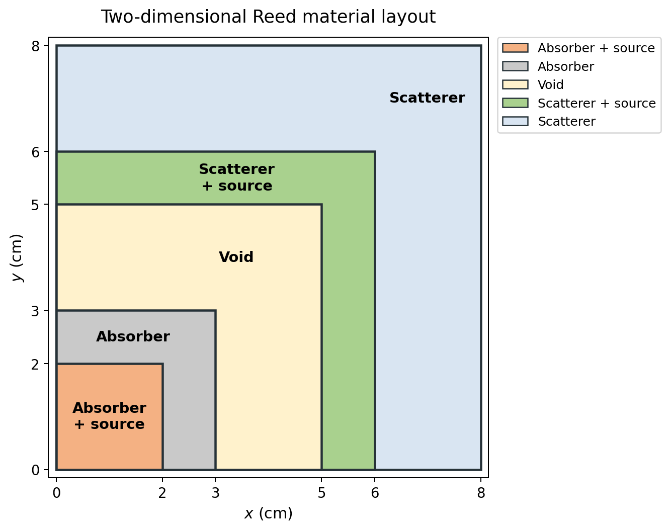
This problem extends the one-dimensional Reed material sequence into a square. The innermost region is a source-bearing absorber, and each subsequent material forms an L-shaped shell around it. The cross sections and source strengths are unchanged from the one-dimensional Reed problem.

3.1.3.1. Import the OpenSn objects

if "opensn_console" not in globals():
    from mpi4py import MPI
    from pyopensn.aquad import GLCProductQuadrature2DXY
    from pyopensn.context import Finalize, UseColor
    from pyopensn.fieldfunc import FieldFunctionInterpolationVolume
    from pyopensn.logvol import RPPLogicalVolume
    from pyopensn.mesh import OrthogonalMeshGenerator
    from pyopensn.solver import DiscreteOrdinatesProblem, SteadyStateSourceSolver
    from pyopensn.source import VolumetricSource
    from pyopensn.xs import MultiGroupXS

    rank = MPI.COMM_WORLD.rank
    UseColor(False)

3.1.3.2. Create the two-dimensional mesh

The domain is the square \([0,8]\times[0,8]\) cm. A uniform spacing of 0.1 cm gives 80 cells along each axis, with nodes at every material interface: 2, 3, 5, and 6 cm.

domain_length = 8.0
cells_per_cm = 10
num_cells = int(domain_length * cells_per_cm)
nodes = [i / cells_per_cm for i in range(num_cells + 1)]

mesh = OrthogonalMeshGenerator(node_sets=[nodes, nodes]).Execute()
mesh.SetOrthogonalBoundaries()

3.1.3.3. Construct the nested material zones

The material at \((x,y)\) is determined by \(\max(x,y)\). Consequently, the first material occupies a square and each later material occupies the difference between two nested squares:

Block ID	Coordinate range	Region	\(\sigma_t\) (cm\(^{-1}\))	\(\sigma_s\) (cm\(^{-1}\))	\(Q\)
0	\(0\leq\max(x,y)\leq2\)	absorber and source	50	0	50
1	\(2<\max(x,y)\leq3\)	absorber	5	0	0
2	\(3<\max(x,y)\leq5\)	void	0	0	0
3	\(5<\max(x,y)\leq6\)	scatterer and source	1	0.9	1
4	\(6<\max(x,y)\leq8\)	scatterer	1	0.9	0

The block IDs are assigned from the outside inward. Each smaller square overwrites the block ID of the cells it contains, leaving the preceding material as an L-shaped shell.

zone_outer_edges = [2.0, 3.0, 5.0, 6.0, 8.0]
mesh.SetUniformBlockID(4)

for block_id, upper_edge in reversed(
    list(enumerate(zone_outer_edges[:-1]))
):
    nested_square = RPPLogicalVolume(
        xmin=0.0, xmax=upper_edge,
        ymin=0.0, ymax=upper_edge,
        infz=True,
    )
    mesh.SetBlockIDFromLogicalVolume(nested_square, block_id, True)

3.1.3.4. Define the materials and sources

As in the one-dimensional problem, CreateSimpleOneGroup receives the total cross section and scattering ratio \(c=\sigma_s/\sigma_t\). The two volumetric sources select the source-bearing regions by block ID.

sigma_t = [50.0, 5.0, 0.0, 1.0, 1.0]
scattering_ratio = [0.0, 0.0, 0.0, 0.9, 0.9]
xs_map = []

for block_id, (total, ratio) in enumerate(
    zip(sigma_t, scattering_ratio)
):
    xs = MultiGroupXS()
    xs.CreateSimpleOneGroup(sigma_t=total, c=ratio)
    xs_map.append({"block_ids": [block_id], "xs": xs})

absorber_source = VolumetricSource(
    block_ids=[0], group_strength=[50.0]
)
scattering_source = VolumetricSource(
    block_ids=[3], group_strength=[1.0]
)

3.1.3.5. Assemble and solve the transport problem

A Gauss–Legendre–Chebyshev quadrature represents directions in the \(xy\) plane. All four exterior faces are vacuum boundaries, preserving the leakage behavior of the one-dimensional problem while allowing particles to stream in two dimensions.

quadrature = GLCProductQuadrature2DXY(
    n_polar=2, n_azimuthal=32, scattering_order=0
)

problem = DiscreteOrdinatesProblem(
    mesh=mesh,
    num_groups=1,
    groupsets=[
        {
            "groups_from_to": (0, 0),
            "angular_quadrature": quadrature,
            "inner_linear_method": "petsc_gmres",
            "l_abs_tol": 1.0e-9,
            "l_max_its": 300,
            "gmres_restart_interval": 30,
        }
    ],
    xs_map=xs_map,
    volumetric_sources=[absorber_source, scattering_source],
    boundary_conditions=[
        {"name": "xmin", "type": "vacuum"},
        {"name": "xmax", "type": "vacuum"},
        {"name": "ymin", "type": "vacuum"},
        {"name": "ymax", "type": "vacuum"},
    ],
)

solver = SteadyStateSourceSolver(problem=problem, compute_balance=True)
solver.Initialize()
solver.Execute()

3.1.3.6. Verify the solution and source geometry

The source-bearing absorber has area \(2^2=4\) cm\(^2\), while the source-bearing scattering shell has area \(6^2-5^2=11\) cm\(^2\). Their strengths therefore give an integrated source rate of \(50(4)+1(11)=211\). The transport balance and maximum scalar flux provide checks on the geometry and computed solution.

balance = solver.ComputeBalanceTable()
source_rate = balance["production_rate"] + balance["inflow_rate"]
loss_rate = balance["absorption_rate"] + balance["outflow_rate"]
relative_balance_error = abs(source_rate - loss_rate) / source_rate

scalar_flux = problem.GetScalarFluxFieldFunction()[0]
whole_domain = RPPLogicalVolume(
    xmin=0.0, xmax=domain_length,
    ymin=0.0, ymax=domain_length,
    infz=True,
)
maximum = FieldFunctionInterpolationVolume()
maximum.SetOperationType("max")
maximum.SetLogicalVolume(whole_domain)
maximum.AddFieldFunction(scalar_flux)
maximum.Execute()
maximum_flux = maximum.GetValue()

if rank == 0:
    print(f"REED_2D_SOURCE_RATE={source_rate:.8e}")
    print(f"REED_2D_MAX_FLUX={maximum_flux:.8e}")
    print(f"REED_2D_BALANCE_ERROR={relative_balance_error:.8e}")

assert abs(source_rate - 211.0) < 1.0e-8
assert relative_balance_error < 1.0e-8

3.1.3.7. Export and visualize the scalar flux

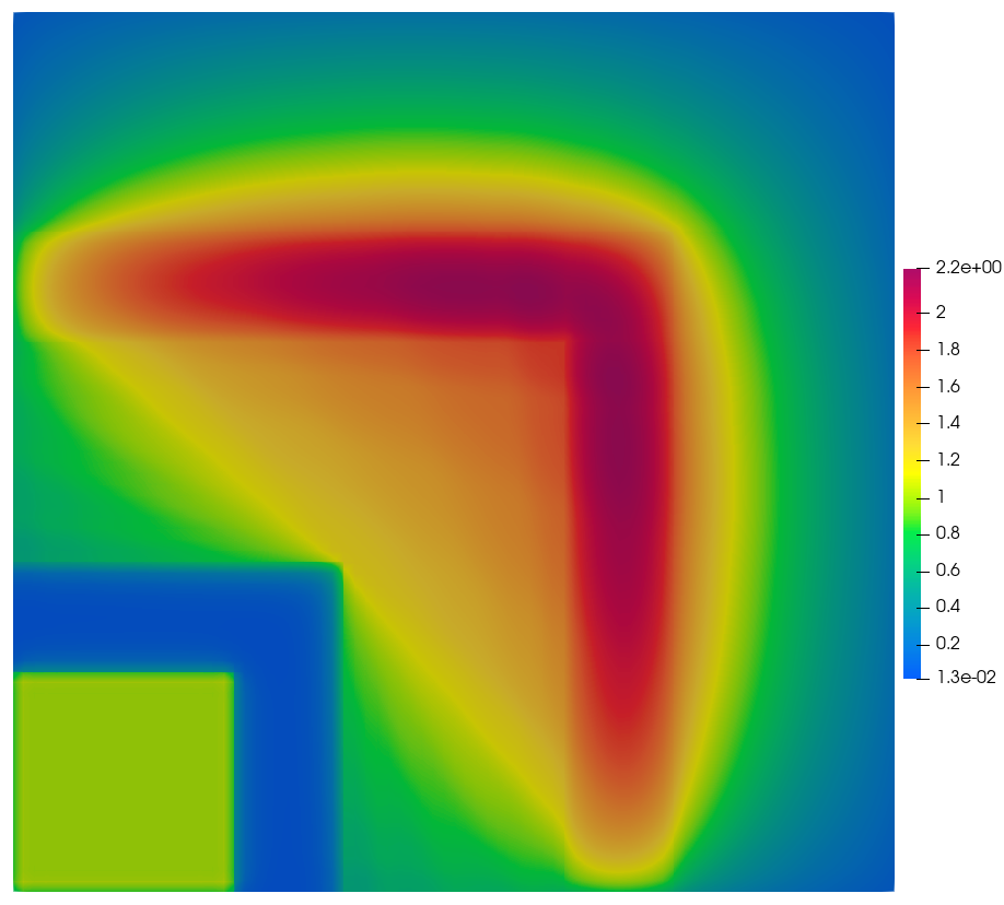
After running the generated Python input, use the following code to export the scalar flux for visualization. It is kept in Markdown so the regression test does not create output files.

from pyopensn.fieldfunc import FieldFunctionGridBased

FieldFunctionGridBased.ExportMultipleToPVTU(
    [scalar_flux], "Flux/Reed2D_Phi"
)

3.1.3.8. Next steps

Compare diagonal and axis-aligned slices of the two-dimensional solution with the one-dimensional Reed flux. You can also refine the mesh near the absorber and void interfaces or increase the azimuthal quadrature to study ray effects.

if "opensn_console" not in globals():
    from IPython import get_ipython

    if get_ipython() is not None:
        Finalize()
        MPI.Finalize()