3.1.6. Shielding with Void and Scattering Regions

This two-dimensional fixed-source problem combines a source, two shielding regions, a near-void, and a highly scattering material. It illustrates how material placement controls the paths by which particles are absorbed or leak through the vacuum boundary.

3.1.6.1. Import the OpenSn objects

if "opensn_console" not in globals():
    from mpi4py import MPI
    from pyopensn.aquad import GLCProductQuadrature2DXY
    from pyopensn.context import Finalize, UseColor
    from pyopensn.logvol import RPPLogicalVolume
    from pyopensn.mesh import OrthogonalMeshGenerator
    from pyopensn.post import VolumePostprocessor
    from pyopensn.solver import DiscreteOrdinatesProblem, SteadyStateSourceSolver
    from pyopensn.source import VolumetricSource
    from pyopensn.xs import MultiGroupXS

    rank = MPI.COMM_WORLD.rank
    UseColor(False)

3.1.6.2. Create the mesh

The domain is \([0,5]\times[0,4]\) cm. The horizontal material interface is at \(y=4/3\) cm. Twelve cells per centimeter align the Cartesian mesh with the integer and one-third-centimeter interfaces. The two-dimensional calculation represents a unit thickness in the \(z\) direction.

width = 5.0
height = 4.0
cells_per_cm = 12
x_nodes = [i / cells_per_cm for i in range(int(width * cells_per_cm) + 1)]
y_nodes = [i / cells_per_cm for i in range(int(height * cells_per_cm) + 1)]

mesh = OrthogonalMeshGenerator(node_sets=[x_nodes, y_nodes]).Execute()
mesh.SetOrthogonalBoundaries()

3.1.6.3. Assign the material regions

The source fills the leftmost strip. Above \(y=4/3\) cm, a one-centimeter-wide shield precedes the scattering region. Below this interface, particles can stream through the near-void before reaching a second shield.

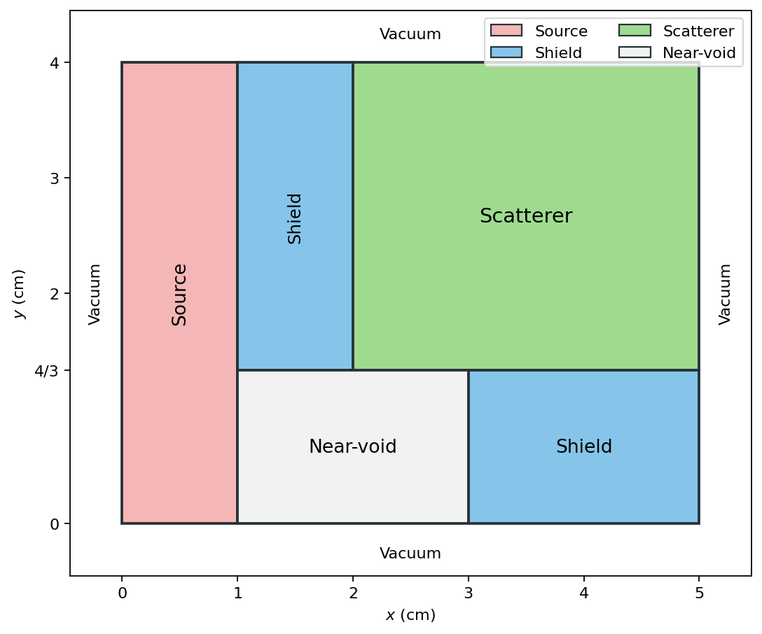
The two disconnected shielding rectangles share one block ID because they use the same cross sections.

SOURCE = 0
SHIELD = 1
SCATTERER = 2
VOID = 3
horizontal_interface = 4.0 / 3.0

mesh.SetUniformBlockID(SOURCE)

regions = [
    (SHIELD, 1.0, 2.0, horizontal_interface, height),
    (SCATTERER, 2.0, width, horizontal_interface, height),
    (VOID, 1.0, 3.0, 0.0, horizontal_interface),
    (SHIELD, 3.0, width, 0.0, horizontal_interface),
]

for block_id, xmin, xmax, ymin, ymax in regions:
    region = RPPLogicalVolume(
        xmin=xmin, xmax=xmax,
        ymin=ymin, ymax=ymax,
        infz=True,
    )
    mesh.SetBlockIDFromLogicalVolume(region, block_id, True)

3.1.6.4. Define the materials and source

CreateSimpleOneGroup receives the total cross section \(\sigma_t\) and scattering ratio \(c=\sigma_s/\sigma_t\). The near-void retains a small total cross section rather than using an exact zero.

Material	\(\sigma_t\) (cm\(^{-1}\))	\(c\)	\(\sigma_s\) (cm\(^{-1}\))	Source (cm\(^{-3}\) s\(^{-1}\))
Source	1.0	0.0	0.0	1.0
Shield	100.0	0.0	0.0	0.0
Scatterer	10.0	0.9999	9.999	0.0
Near-void	0.001	0.0	0.0	0.0

The volumetric source is applied only to the left strip.

material_data = [
    (SOURCE, 1.0, 0.0),
    (SHIELD, 100.0, 0.0),
    (SCATTERER, 10.0, 0.9999),
    (VOID, 0.001, 0.0),
]

xs_map = []
for block_id, sigma_t, scattering_ratio in material_data:
    xs = MultiGroupXS()
    xs.CreateSimpleOneGroup(sigma_t=sigma_t, c=scattering_ratio)
    xs_map.append({"block_ids": [block_id], "xs": xs})

source = VolumetricSource(
    block_ids=[SOURCE], group_strength=[1.0]
)

3.1.6.5. Assemble and solve the transport problem

A Gauss–Legendre–Chebyshev quadrature represents directions in the \(xy\) plane. All exterior faces are vacuum boundaries. The tight linear tolerance is useful here because the scattering region has a scattering ratio close to one.

quadrature = GLCProductQuadrature2DXY(
    n_polar=2, n_azimuthal=64, scattering_order=0
)

problem = DiscreteOrdinatesProblem(
    mesh=mesh,
    num_groups=1,
    groupsets=[
        {
            "groups_from_to": (0, 0),
            "angular_quadrature": quadrature,
            "inner_linear_method": "petsc_gmres",
            "l_abs_tol": 1.0e-9,
            "l_max_its": 400,
            "gmres_restart_interval": 40,
        }
    ],
    xs_map=xs_map,
    volumetric_sources=[source],
    boundary_conditions=[
        {"name": "xmin", "type": "vacuum"},
        {"name": "xmax", "type": "vacuum"},
        {"name": "ymin", "type": "vacuum"},
        {"name": "ymax", "type": "vacuum"},
    ],
)

solver = SteadyStateSourceSolver(problem=problem, compute_balance=True)
solver.Initialize()
solver.Execute()

3.1.6.6. Check the flux and particle balance

The source strip has area \(1\times4=4\) cm\(^2\), giving an integrated source rate of 4 particles per second per unit depth. We compute the average scalar flux in the highly scattering region and the absorption rate in the two shielding regions. These quantities exercise both the material layout and the transport solution.

scatterer_flux_postprocessor = VolumePostprocessor(
    problem=problem, value_type="avg", block_ids=[SCATTERER]
)
scatterer_flux_postprocessor.Execute()
scatterer_average_flux = scatterer_flux_postprocessor.GetValue()[0][0]

shield_absorption_postprocessor = VolumePostprocessor(
    problem=problem,
    value_type="integral",
    block_ids=[SHIELD],
    xs_multiplier="sigma_a",
)
shield_absorption_postprocessor.Execute()
shield_absorption_rate = shield_absorption_postprocessor.GetValue()[0][0]

balance = solver.ComputeBalanceTable()
source_rate = balance["production_rate"] + balance["inflow_rate"]
loss_rate = balance["absorption_rate"] + balance["outflow_rate"]
relative_balance_error = abs(source_rate - loss_rate) / source_rate

if rank == 0:
    print(f"SHIELDING_SOURCE_RATE={source_rate:.8e}")
    print(f"SHIELDING_SCATTERER_AVG_FLUX={scatterer_average_flux:.8e}")
    print(f"SHIELDING_ABSORPTION_RATE={shield_absorption_rate:.8e}")
    print(f"SHIELDING_BALANCE_ERROR={relative_balance_error:.8e}")

assert abs(source_rate - 4.0) < 1.0e-8
assert relative_balance_error < 1.0e-8

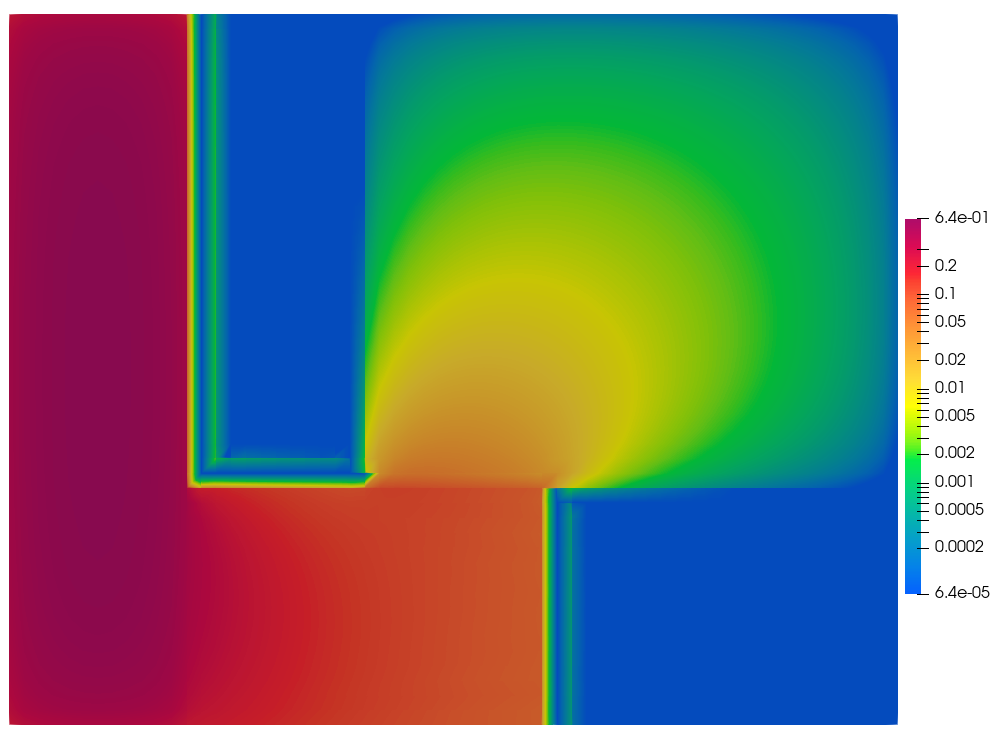
3.1.6.7. Export and visualize the scalar flux

After running the generated Python input, use the following code to export the scalar flux for visualization. It is kept in Markdown so the regression test does not create output files.

from pyopensn.fieldfunc import FieldFunctionGridBased

scalar_flux = problem.GetScalarFluxFieldFunction()[0]
FieldFunctionGridBased.ExportMultipleToPVTU(
    [scalar_flux], "Flux/ShieldingWithVoid_Phi"
)

3.1.6.8. Next steps

Compare transport through the near-void and shielding paths, refine the mesh in the optically thick shield, or increase the azimuthal resolution to study ray effects.

if "opensn_console" not in globals():
    from IPython import get_ipython

    if get_ipython() is not None:
        Finalize()
        MPI.Finalize()