3.1.8. A Three-Dimensional Volumetric-Source Problem

This example solves a steady, one-group transport problem on a three-dimensional Cartesian mesh containing separate background, source, and detector materials. An isotropic volumetric source is confined to a scattering material, particles travel through a predominantly scattering background, and the detector response is evaluated in an absorbing region. All material, source, mesh, and solver parameters are defined in the input, so the example requires no command-line parameters or interactive input.

3.1.8.1. Import the OpenSn objects

if "opensn_console" not in globals():
    from mpi4py import MPI
    from pyopensn.aquad import GLCProductQuadrature3DXYZ
    from pyopensn.context import Finalize, UseColor
    from pyopensn.fieldfunc import FieldFunctionInterpolationVolume
    from pyopensn.logvol import RPPLogicalVolume
    from pyopensn.mesh import OrthogonalMeshGenerator
    from pyopensn.solver import DiscreteOrdinatesProblem, SteadyStateSourceSolver
    from pyopensn.source import VolumetricSource
    from pyopensn.xs import MultiGroupXS

    rank = MPI.COMM_WORLD.rank
    UseColor(False)

3.1.8.2. Create the three-dimensional mesh

Supplying three node sets creates a Cartesian mesh in \(x\), \(y\), and \(z\). The nodes align the mesh with every source and detector interface in the 10-by-10-by-10 domain, with two cells across each coordinate interval.

nodes = [
    0.0, 1.0, 2.0, 2.5, 3.0, 3.5, 4.0, 5.0,
    6.0, 7.0, 8.0, 8.25, 8.5, 9.25, 10.0,
]

mesh = OrthogonalMeshGenerator(node_sets=[nodes, nodes, nodes]).Execute()
mesh.SetOrthogonalBoundaries()

BACKGROUND_MATERIAL = 0
SOURCE_MATERIAL = 1
DETECTOR_MATERIAL = 2
mesh.SetUniformBlockID(BACKGROUND_MATERIAL)

3.1.8.3. Define the material and source regions

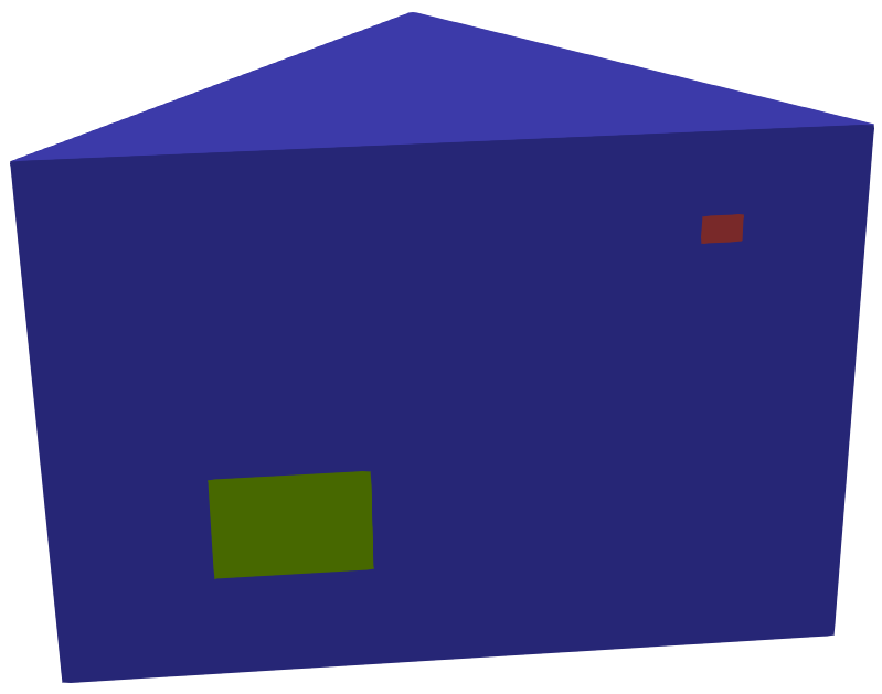
The source is confined to the cube from 2 to 4 along each axis. The much smaller detector occupies the cube from 8 to 8.5. These logical volumes assign distinct material IDs to the two regions while the rest of the domain remains the background material.

source_region = RPPLogicalVolume(
    xmin=2.0, xmax=4.0,
    ymin=2.0, ymax=4.0,
    zmin=2.0, zmax=4.0,
)
detector_region = RPPLogicalVolume(
    xmin=8.0, xmax=8.5,
    ymin=8.0, ymax=8.5,
    zmin=8.0, zmax=8.5,
)

mesh.SetBlockIDFromLogicalVolume(source_region, SOURCE_MATERIAL, True)
mesh.SetBlockIDFromLogicalVolume(detector_region, DETECTOR_MATERIAL, True)

background_xs = MultiGroupXS()
background_xs.CreateSimpleOneGroup(sigma_t=1.0, c=0.9)

source_xs = MultiGroupXS()
source_xs.CreateSimpleOneGroup(sigma_t=2.0, c=1.0)

detector_sigma_t = 0.8
detector_xs = MultiGroupXS()
detector_xs.CreateSimpleOneGroup(sigma_t=detector_sigma_t, c=0.0)

source_volume = (4.0 - 2.0) ** 3
source = VolumetricSource(
    block_ids=[SOURCE_MATERIAL],
    group_strength=[1.0 / source_volume],
)

3.1.8.4. Assemble and solve the transport problem

A three-dimensional product quadrature represents particle directions over the sphere. Vacuum conditions on all six faces allow particles to leave the cube. The source strength is normalized by its volume so that the integrated source rate is one particle per unit time.

quadrature = GLCProductQuadrature3DXYZ(
    n_polar=8,
    n_azimuthal=8,
    scattering_order=0,
)

problem = DiscreteOrdinatesProblem(
    mesh=mesh,
    num_groups=1,
    groupsets=[
        {
            "groups_from_to": (0, 0),
            "angular_quadrature": quadrature,
            "inner_linear_method": "petsc_gmres",
            "l_abs_tol": 1.0e-10,
            "l_max_its": 200,
            "gmres_restart_interval": 30,
        }
    ],
    xs_map=[
        {"block_ids": [BACKGROUND_MATERIAL], "xs": background_xs},
        {"block_ids": [SOURCE_MATERIAL], "xs": source_xs},
        {"block_ids": [DETECTOR_MATERIAL], "xs": detector_xs},
    ],
    volumetric_sources=[source],
    boundary_conditions=[
        {"name": "xmin", "type": "vacuum"},
        {"name": "xmax", "type": "vacuum"},
        {"name": "ymin", "type": "vacuum"},
        {"name": "ymax", "type": "vacuum"},
        {"name": "zmin", "type": "vacuum"},
        {"name": "zmax", "type": "vacuum"},
    ],
)

solver = SteadyStateSourceSolver(problem=problem)
solver.Initialize()
solver.Execute()

3.1.8.5. Evaluate the detector response

The volume interpolation integrates the scalar flux over the detector. Multiplication by the detector’s total interaction cross section produces its response. This single deterministic value also makes the example suitable for regression testing.

scalar_flux = problem.GetScalarFluxFieldFunction()[0]
response = FieldFunctionInterpolationVolume()
response.SetOperationType("sum")
response.SetLogicalVolume(detector_region)
response.AddFieldFunction(scalar_flux)
response.Execute()
response_value = detector_sigma_t * response.GetValue()

if rank == 0:
    print(f"FIXED_SOURCE_3D_RESPONSE={response_value:.8e}")

3.1.8.6. Visualize the scalar flux

from pyopensn.fieldfunc import FieldFunctionGridBased

fflist = problem.GetScalarFluxFieldFunction()
FieldFunctionGridBased.ExportMultipleToPVTU(
    [fflist[0]], "Flux/Phi_p"
)

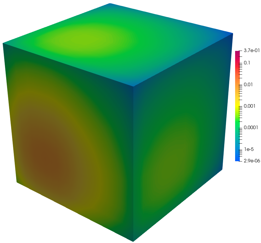
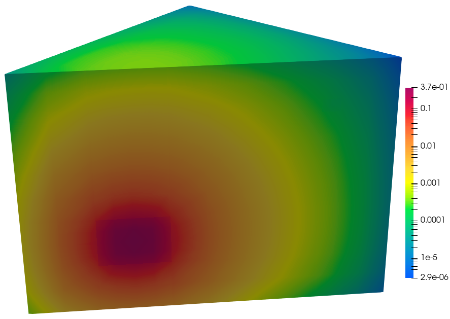
The resulting scalar-flux distribution is shown below.

3.1.8.7. Next steps

Try refining each coordinate interval, changing the background material, or moving the source and detector regions. Because every parameter is set above, the notebook and its generated Python input can be run without supplying environment variables or other terminal-level inputs.

if "opensn_console" not in globals():
    from IPython import get_ipython

    if get_ipython() is not None:
        Finalize()
        MPI.Finalize()