3.1.7. A Striped Fixed-Source Problem

This two-dimensional problem places three source-bearing material stripes in a scattering background. Two reflecting boundaries reproduce neighboring copies of the modeled quadrant, while particles can escape through the top and right vacuum boundaries.

3.1.7.1. Import the OpenSn objects

import csv
import os
from glob import glob

import matplotlib.pyplot as plt

if "opensn_console" not in globals():
    from mpi4py import MPI
    from pyopensn.aquad import GLCProductQuadrature2DXY
    from pyopensn.context import Finalize, UseColor
    from pyopensn.fieldfunc import FieldFunctionInterpolationLine
    from pyopensn.logvol import RPPLogicalVolume
    from pyopensn.math import Vector3
    from pyopensn.mesh import OrthogonalMeshGenerator
    from pyopensn.post import VolumePostprocessor
    from pyopensn.solver import DiscreteOrdinatesProblem, SteadyStateSourceSolver
    from pyopensn.source import VolumetricSource
    from pyopensn.xs import MultiGroupXS

    comm = MPI.COMM_WORLD
    rank = comm.rank
    barrier = comm.Barrier
    UseColor(False)
else:
    rank = 0
    barrier = MPIBarrier

3.1.7.2. Create the mesh

The domain is \([0,10]\times[0,10]\) cm. A uniform spacing of 0.1 cm places mesh nodes on every stripe edge and on the horizontal interface at \(y=9\) cm. The two-dimensional calculation represents a unit thickness in the \(z\) direction.

domain_length = 10.0
cells_per_cm = 10
num_cells = int(domain_length * cells_per_cm)
nodes = [i / cells_per_cm for i in range(num_cells + 1)]

mesh = OrthogonalMeshGenerator(node_sets=[nodes, nodes]).Execute()
mesh.SetOrthogonalBoundaries()

3.1.7.3. Assign the material stripes

Material M fills the domain. Three F regions occupy \(1\leq x\leq2\), \(4\leq x\leq5\), and \(7\leq x\leq8\) cm, each extending from \(y=0\) to \(y=9\) cm.

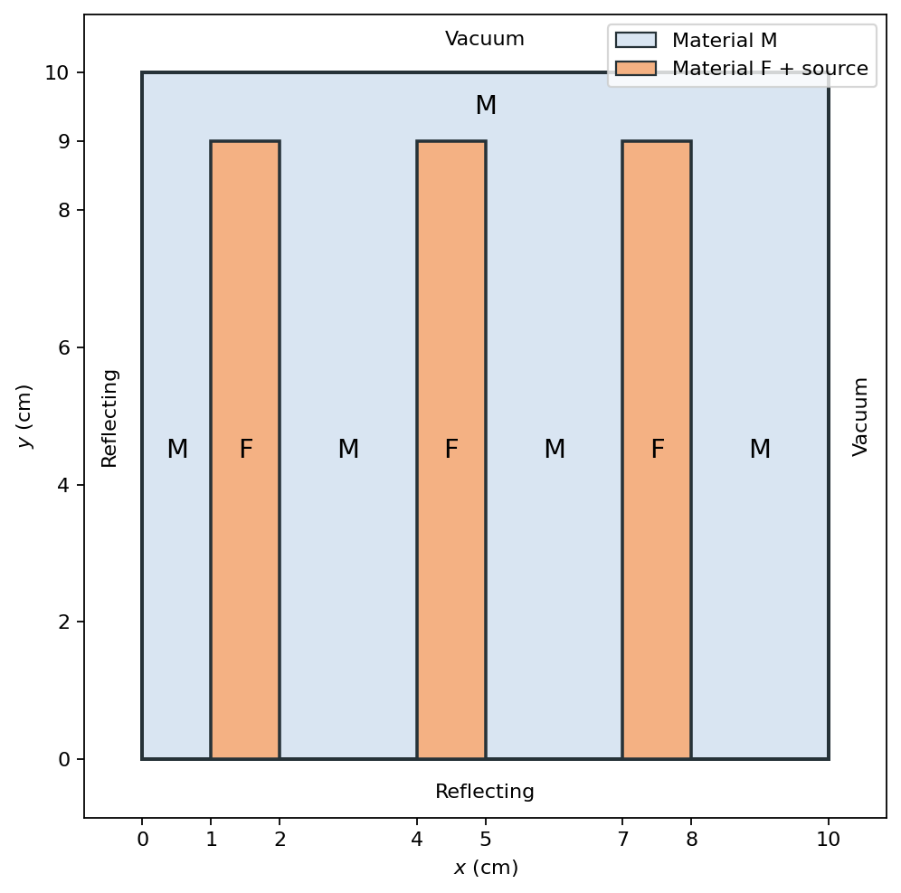
The F regions share one block ID, allowing a single material definition and source to be applied to all three disconnected stripes.

MATERIAL_M = 0
MATERIAL_F = 1
stripe_intervals = [(1.0, 2.0), (4.0, 5.0), (7.0, 8.0)]

mesh.SetUniformBlockID(MATERIAL_M)

for xmin, xmax in stripe_intervals:
    stripe = RPPLogicalVolume(
        xmin=xmin, xmax=xmax,
        ymin=0.0, ymax=9.0,
        infz=True,
    )
    mesh.SetBlockIDFromLogicalVolume(stripe, MATERIAL_F, True)

3.1.7.4. Define the materials and source

This tutorial uses the total and isotropic-scattering cross sections from the reference material table. The tabulated fission terms for material F are deliberately set to zero, and a unit external source is applied to the F stripes instead.

Material	\(\sigma_t\) (cm\(^{-1}\))	\(\sigma_{s0}\) (cm\(^{-1}\))	\(c=\sigma_{s0}/\sigma_t\)	External source (cm\(^{-3}\) s\(^{-1}\))
M	1.0	0.93	0.93	0.0
F	1.5	1.35	0.90	1.0

Because CreateSimpleOneGroup creates non-fissile one-group data, no fission source is present in either material.

xs_m = MultiGroupXS()
xs_m.CreateSimpleOneGroup(sigma_t=1.0, c=0.93)

xs_f = MultiGroupXS()
xs_f.CreateSimpleOneGroup(sigma_t=1.5, c=1.35 / 1.5)

source = VolumetricSource(
    block_ids=[MATERIAL_F], group_strength=[1.0]
)

3.1.7.5. Assemble and solve the transport problem

The xmin and ymin faces are reflecting, while xmax and ymax are vacuum. A Gauss–Legendre–Chebyshev quadrature represents directions in the \(xy\) plane.

quadrature = GLCProductQuadrature2DXY(
    n_polar=2, n_azimuthal=32, scattering_order=0
)

problem = DiscreteOrdinatesProblem(
    mesh=mesh,
    num_groups=1,
    groupsets=[
        {
            "groups_from_to": (0, 0),
            "angular_quadrature": quadrature,
            "inner_linear_method": "petsc_gmres",
            "l_abs_tol": 1.0e-9,
            "l_max_its": 300,
            "gmres_restart_interval": 30,
        }
    ],
    xs_map=[
        {"block_ids": [MATERIAL_M], "xs": xs_m},
        {"block_ids": [MATERIAL_F], "xs": xs_f},
    ],
    volumetric_sources=[source],
    boundary_conditions=[
        {"name": "xmin", "type": "reflecting"},
        {"name": "xmax", "type": "vacuum"},
        {"name": "ymin", "type": "reflecting"},
        {"name": "ymax", "type": "vacuum"},
    ],
)

solver = SteadyStateSourceSolver(problem=problem, compute_balance=True)
solver.Initialize()
solver.Execute()

3.1.7.6. Check the source and particle balance

Each F stripe has area \(1\times9=9\) cm\(^2\). The three unit-strength source regions therefore produce 27 particles per second per unit depth. We also compute the average scalar flux and absorption rate over the combined F-region block ID.

production_rate measures the external volumetric source. The balance table also reports particles leaving and reentering through reflecting faces as outflow and inflow, respectively, so the complete balance includes both boundary terms.

f_flux_postprocessor = VolumePostprocessor(
    problem=problem, value_type="avg", block_ids=[MATERIAL_F]
)
f_flux_postprocessor.Execute()
f_region_average_flux = f_flux_postprocessor.GetValue()[0][0]

f_absorption_postprocessor = VolumePostprocessor(
    problem=problem,
    value_type="integral",
    block_ids=[MATERIAL_F],
    xs_multiplier="sigma_a",
)
f_absorption_postprocessor.Execute()
f_region_absorption_rate = f_absorption_postprocessor.GetValue()[0][0]

balance = solver.ComputeBalanceTable()
external_source_rate = balance["production_rate"]
total_gain_rate = external_source_rate + balance["inflow_rate"]
loss_rate = balance["absorption_rate"] + balance["outflow_rate"]
relative_balance_error = abs(total_gain_rate - loss_rate) / total_gain_rate

if rank == 0:
    print(f"STRIPED_SOURCE_RATE={external_source_rate:.8e}")
    print(f"STRIPED_SOURCE_AVG_FLUX={f_region_average_flux:.8e}")
    print(f"STRIPED_SOURCE_ABSORPTION_RATE={f_region_absorption_rate:.8e}")
    print(f"STRIPED_SOURCE_BALANCE_ERROR={relative_balance_error:.8e}")

assert abs(external_source_rate - 27.0) < 1.0e-8
assert relative_balance_error < 1.0e-8

3.1.7.7. Sample the flux along the horizontal centerline

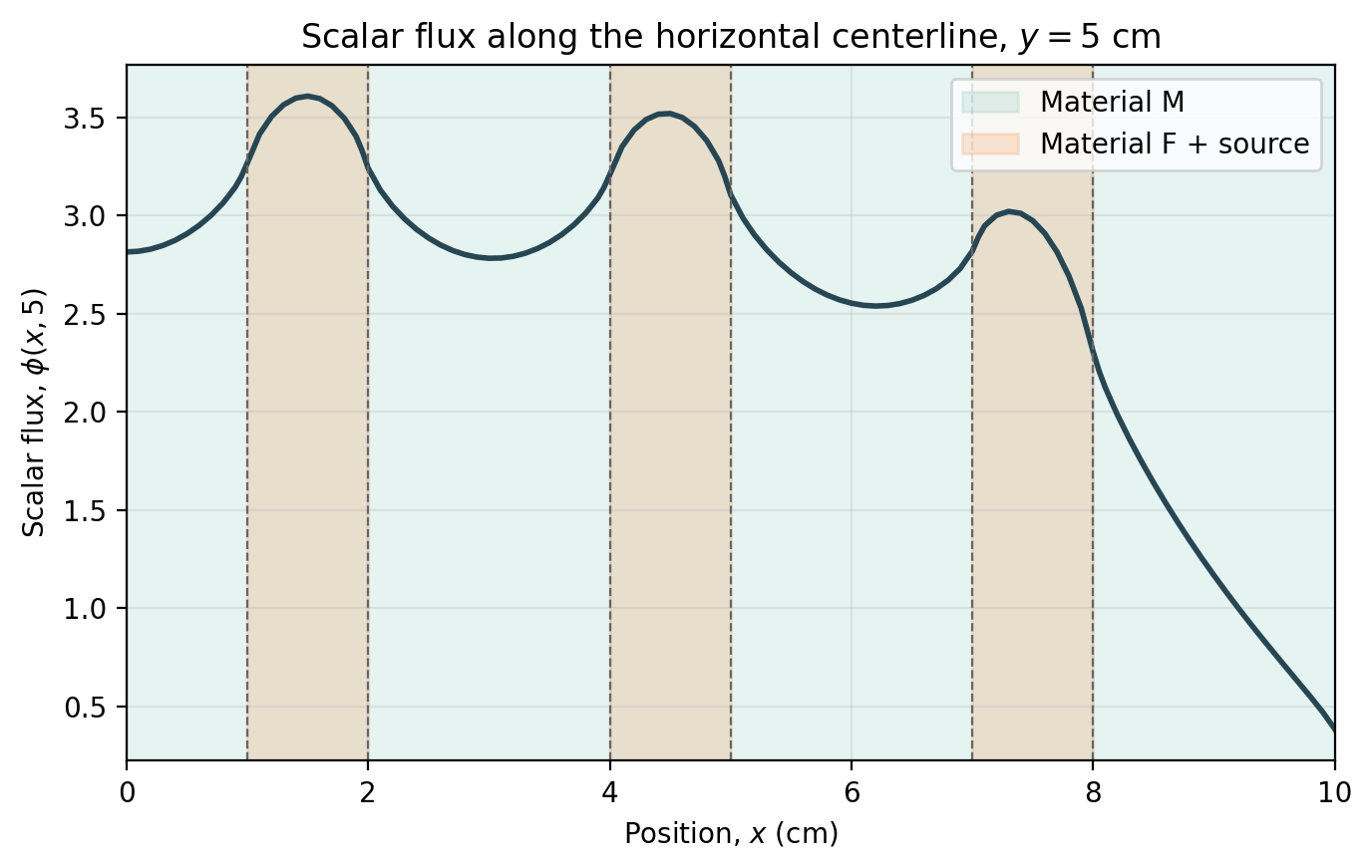
A FieldFunctionInterpolationLine samples the scalar flux from left to right at \(y=5\) cm, crossing all three source stripes. The endpoints are shifted slightly inside the mesh so every one of the 201 sample points has an unambiguous containing cell. ExportToCSV gathers the distributed samples on rank 0; the CSV is read for plotting and then removed to keep regression runs clean.

scalar_flux = problem.GetScalarFluxFieldFunction()[0]
epsilon = 1.0e-6
centerline = FieldFunctionInterpolationLine()
centerline.SetInitialPoint(Vector3(epsilon, 5.0, 0.0))
centerline.SetFinalPoint(Vector3(domain_length - epsilon, 5.0, 0.0))
centerline.SetNumberOfPoints(201)
centerline.AddFieldFunction(scalar_flux)
centerline.Execute()

csv_prefix = "striped_source_centerline"
if rank == 0:
    for old_file in glob(f"{csv_prefix}_*.csv"):
        os.remove(old_file)
barrier()
centerline.ExportToCSV(csv_prefix)
barrier()

centerline_maximum = None
centerline_right_boundary = None
if rank == 0:
    csv_filename = glob(f"{csv_prefix}_*.csv")[0]
    with open(csv_filename, newline="") as csv_file:
        reader = csv.DictReader(csv_file)
        field_column = next(
            name for name in reader.fieldnames if name not in ("x", "y", "z")
        )
        rows = list(reader)
    x = [float(row["x"]) for row in rows]
    centerline_flux = [float(row[field_column]) for row in rows]
    centerline_maximum = max(centerline_flux)
    centerline_right_boundary = centerline_flux[-1]

    fig, ax = plt.subplots(figsize=(7.0, 4.5))
    ax.axvspan(0.0, domain_length, color="#2a9d8f", alpha=0.12, label="Material M")
    for index, (xmin, xmax) in enumerate(stripe_intervals):
        ax.axvspan(
            xmin,
            xmax,
            color="#f4a261",
            alpha=0.25,
            label="Material F + source" if index == 0 else None,
        )
    ax.plot(x, centerline_flux, color="#264653", linewidth=2.0)
    for interface in [value for interval in stripe_intervals for value in interval]:
        ax.axvline(interface, color="0.4", linestyle="--", linewidth=0.8)
    ax.set_xlabel(r"Position, $x$ (cm)")
    ax.set_ylabel(r"Scalar flux, $\phi(x,5)$")
    ax.set_title(r"Scalar flux along the horizontal centerline, $y=5$ cm")
    ax.set_xlim(0.0, domain_length)
    ax.grid(alpha=0.25)
    ax.legend()
    fig.tight_layout()
    # fig.savefig("images/striped_source_centerline.png", dpi=200, bbox_inches="tight")
    plt.close(fig)
    os.remove(csv_filename)

if "opensn_console" not in globals():
    centerline_maximum = comm.bcast(centerline_maximum, root=0)
    centerline_right_boundary = comm.bcast(centerline_right_boundary, root=0)
if rank == 0:
    print(f"STRIPED_SOURCE_LINE_MAX={centerline_maximum:.8e}")
    print(f"STRIPED_SOURCE_LINE_RIGHT={centerline_right_boundary:.8e}")
assert centerline_maximum > centerline_right_boundary > 0.0

The three local maxima align with the source-bearing F stripes. Their heights differ because the left and bottom boundaries are reflecting, whereas particles can leak through the top and right boundaries. The committed figure was generated by the preceding cell; uncomment fig.savefig(...) to regenerate it after changing the problem.

3.1.7.8. Export and visualize the scalar flux

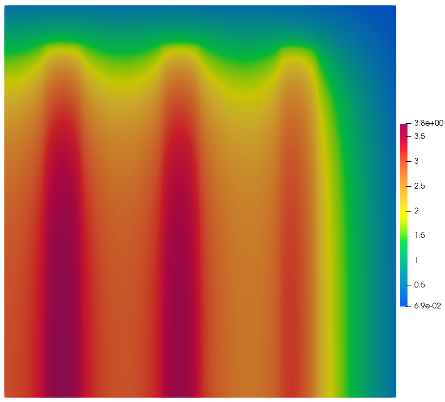
After running the generated Python input, use the following code to export the scalar flux for visualization. It is kept in Markdown so the regression test does not create output files.

from pyopensn.fieldfunc import FieldFunctionGridBased

scalar_flux = problem.GetScalarFluxFieldFunction()[0]
FieldFunctionGridBased.ExportMultipleToPVTU(
    [scalar_flux], "Flux/StripedSource_Phi"
)

3.1.7.9. Next steps

Compare the flux in the three source stripes, replace the external source with the original fission data to recover an eigenvalue problem, or change the reflecting faces to vacuum and examine the resulting leakage.

if "opensn_console" not in globals():
    from IPython import get_ipython

    if get_ipython() is not None:
        Finalize()
        MPI.Finalize()